Lab 07 – Tools for Final Projects

Some Housekeeping Notes:

1. Lab computers:
   • Please do not turn off computers when leaving the lab! They get important updates at night, but only if they are left running (do log out of your personal account, though).
     
2. Lab flexibility:
   • The next three weeks of lab are going to be dedicated to final projects. If you want more lab time to work on your project, you are welcome to drop in to the other GEOG 204 lab sections (Tuesdays, Wednesdays, or Thursdays, 3:00 – 5:50 PM) if there are extra seats.
   • Also don’t forget that you can access the GIS lab in person after hours by following the instructions HERE, or you can access Osmotar from your home computer by following the instructions HERE.
     
3. Tutorials on Monday, November 22:
   • Tutorials on Monday, November 22 will also be dedicated to working on final projects (in your usual classroom), and Anthony will be available for support.

Coordinate Reference Systems & Your Project

Choosing a Coordinate Reference System

It’s important to choose a reference system (CRS) that is relevant to your project’s area of interest, and to project all of your layers to the same CRS (remember, this counts for marks in your final project!) before you begin your analyses.

There are two main things to consider:

1. Your project Coordinate Reference System, and
2. Your layer Coordinate Reference Systems (each individual layer has its own CRS)

Any number of things can go wrong if you have an incorrect projection somewhere! Your data, meant to be in BC, could appear somewhere in the middle of the ocean on the other side of the world, or it could be completely distorted. Have a look at the examples below.

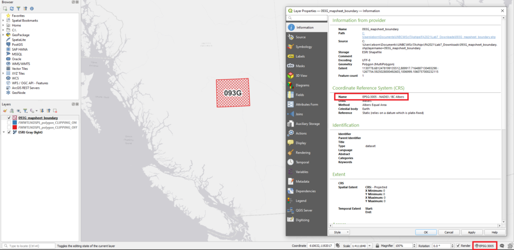
If both your project CRS and your layer CRS match, they’ll be displayed correctly:

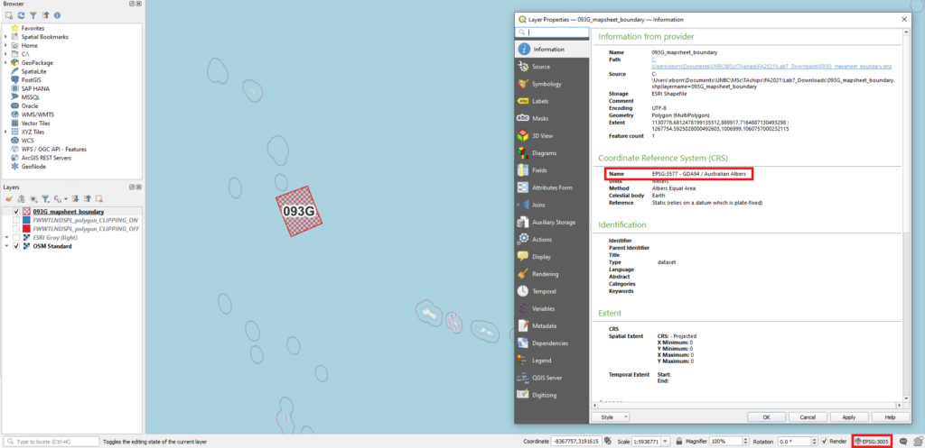
If your layer CRS is wonky, your data won’t be displayed in the right place:

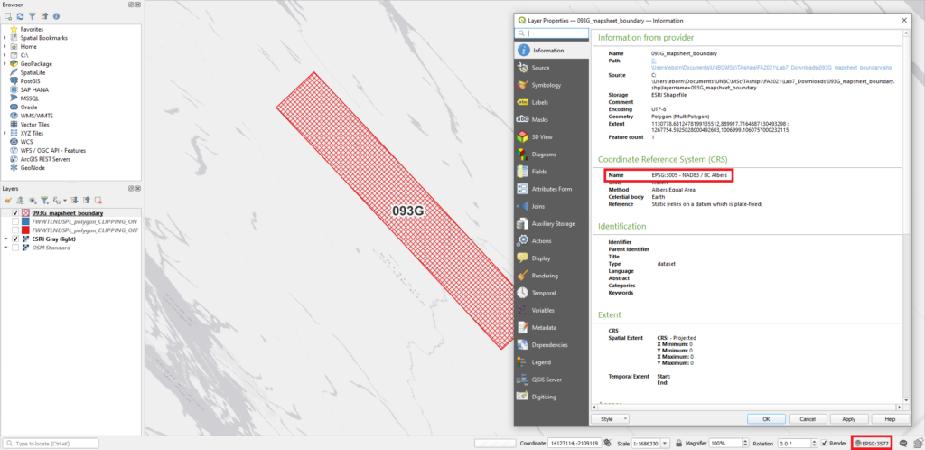
If your project CRS is wonky, your layer will be distorted:

These are extreme examples meant to illustrate what happens when projections don’t match. Another problem you may run into is that things may look correct, but some GIS tools will give an error message if you try to use two layers with different projections.

Reprojecting Layers

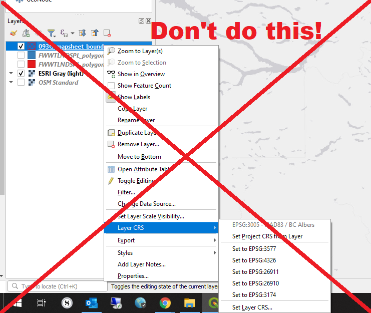
Right click on the layer whose CRS you want to modify, but don’t be fooled by the ‘Layer CRS’ button. This will modify the physical location your data is displayed rather than changing the actual CRS. Modifying the Layer CRS is how I created the error above where the mapsheet is displayed in the ocean.

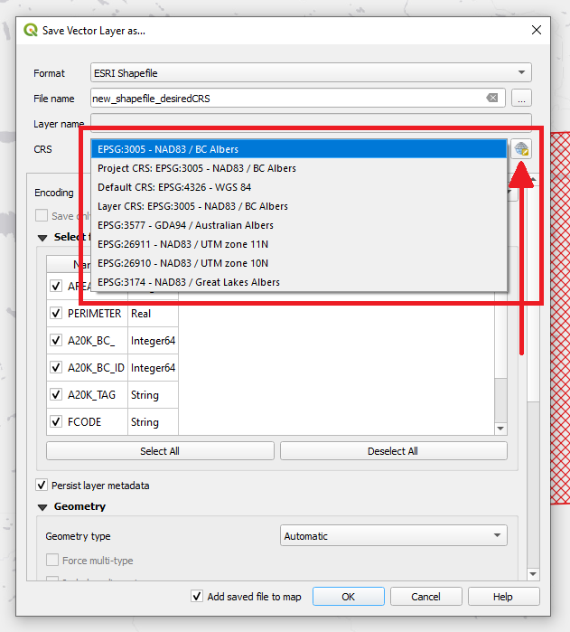
Instead, click Export > Save Features (or Selected Features) As…

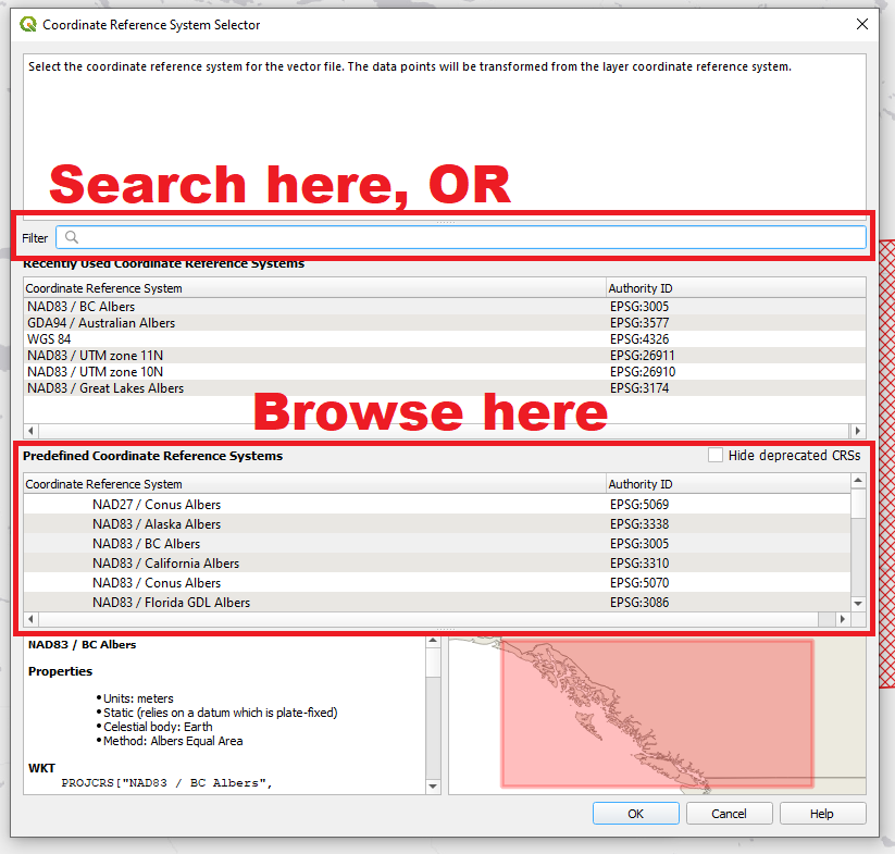
Save your layer as a new shapefile, and set your desired CRS like we’ve done in previous labs. Don’t see the CRS you want in the drop-down list? Click on the globe icon to the right of the drop-down.

What CRS should I use, then?

The answer depends on where your project is based:

• If it’s anywhere in BC, BC Albers (EPSG: 3005) is a good bet;
• The UTM zone that covers your project area works well, and applies anywhere in the world;
• There are many other coordinate reference systems out there that may apply to your project area – search the Coordinate Reference System Selector (pictured above) or online if you want to explore them.

Downloading Content from Data Catalogue BC

For your final project, you can source your spatial data from nearly anywhere. A valuable resource if your area of interest falls within British Columbia, however, is Data Catalogue BC.

Many jurisdictions have similar websites that you can find through a Google search, but we’re going to use DataBC as an example.

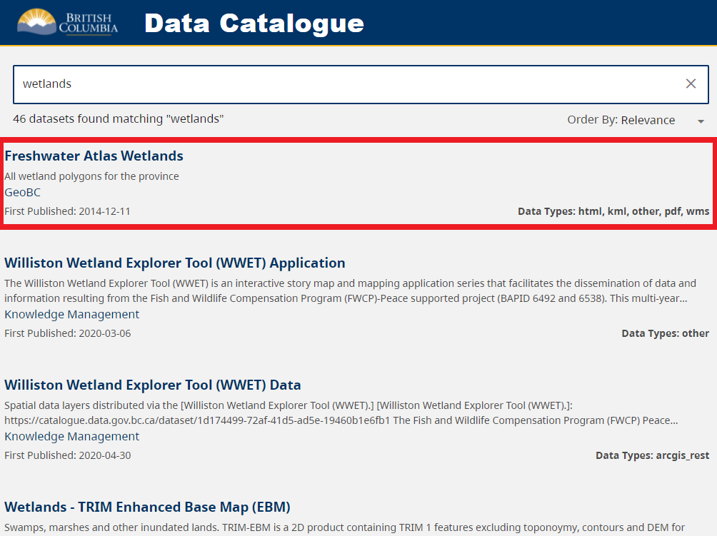
Let’s say I’m looking for the locations of wetlands across BC. Go to Data Catalogue BC and search for wetlands now.

Filtering Results

We can filter the search results to help make the results more relevant. Expand the Download Permissions tab, and select Public. Next, click on Resource Storage Format. Many of these file types will be familiar: CSV, KML, KMZ, SHP, and a few others are all file types that we’ve worked with in class. Let’s select SHP as our file type.

The first search result, Freshwater Atlas Wetlands, is still there at the top of the list of results, so we know that it has Public download permissions, and is available for download in a Shapefile format. There’s also a brief description of the dataset, indicating that it’s a file containing wetland polygons for BC. Click on the Freshwater Atlas Wetlands and we’ll check it out in more detail.

As a side note, there are multiple Freshwater Atlases for BC, including Glaciers, Coastlines, Obstructions, and more – search for ‘Freshwater Atlas’ to see them if they might be useful for your project.

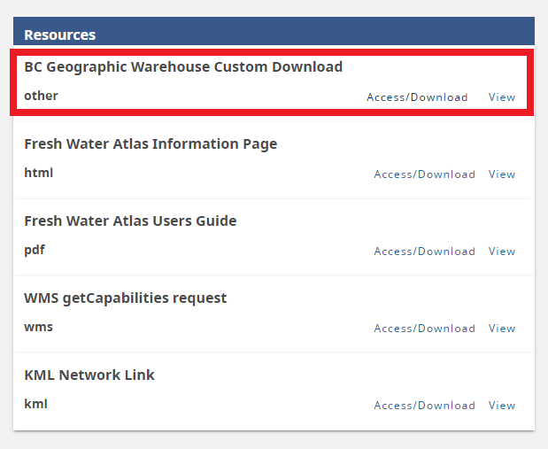
The dataset’s webpage gives us more information about who published it, what the access licence is, what the purpose of the dataset is, and so on. Once we’ve decided that this is the dataset we want to download, let’s go investigate the Resources section:

Downloading Data

The Resources section contains a number of links that may be useful like an Information Page and Users Guide, but let’s go ahead and download the spatial data. Click on the Access/Download button in the BC Geographic Warehouse Custom Download section to open this pop-up:

Specify the Details

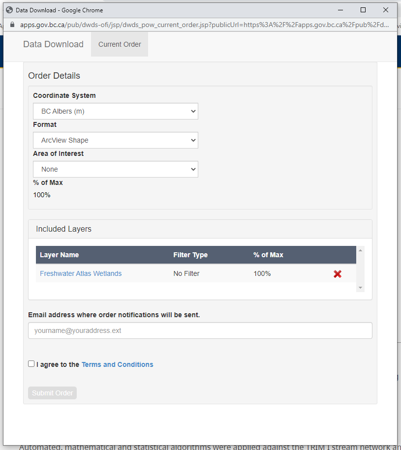
The Data Download window allows you to specify the details of your download. You can choose what Coordinate System you want, the file format you want (choose ArcView Shape for Shapefiles), and your Area of Interest.

Note below that, where it says % of Max: this is referring to the size of your download. Some files are so large that they can’t be downloaded in one go. In those cases, the % of Max will be greater than 100%. Your data download will only work if the ‘% of Max’ is 100% or less.

Often, you don’t want data for all of BC, anyway, so let’s narrow down our area of interest (which reduces our % of Max value). There’s multiple ways to do this:

1. Mapsheet
   • We learned how to find our desired mapsheet back in Lab 6 – refer back to it if you need a refresher on finding which mapsheet you want.
   • Enter your desired mapsheet (remember PG is in mapsheet 93G?) in the space provided, and select Use Mapsheet – your % of Max drops to 3%, which is way more manageable!
2. Draw a Custom AOI
   • If your AOI (Area of Interest) crosses mapsheet boundaries or doesn’t otherwise suit selection by mapsheet, draw a custom AOI. Either:
   • A) Draw a custom AOI within the pop-up window. Click Draw a Custom AOI, then use one of the selection tools to mark out your Area of Interest on the map. Once done (and it shows Geometry captured), click Next. It will give you the choice to add more polygons, remove the polygon you made, or Submit AOI. Submit AOI if you’re happy. OR:
   • B) Upload a .zip file containing a polygon shapefile (remember all those file extensions that have to be included!) that you create yourself in QGIS. You can open up a web map from QuickMapServices for reference, then digitize your own boundary polygon (like the Forests for the World boundary in Lab 4) in a new shapefile layer – refer back to Lab 2 for a refresher on creating new layers.

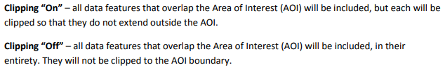
Clipping

Clipping, in this context, refers to whether features will be clipped to the exact boundary you’ve specified or not. It is defined well in the BC Data Catalogue help document here:

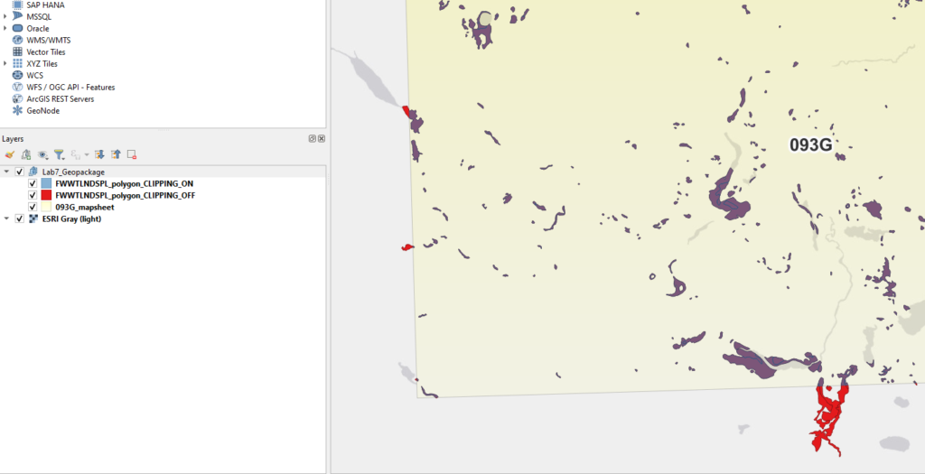
The image above shows two downloads of the same dataset (Freshwater Atlas Wetlands for mapsheet 093G). The blue, semi-transparent layer (looks purple on the map) is with clipping on. The red, opaque layer is with clipping off. See the difference?

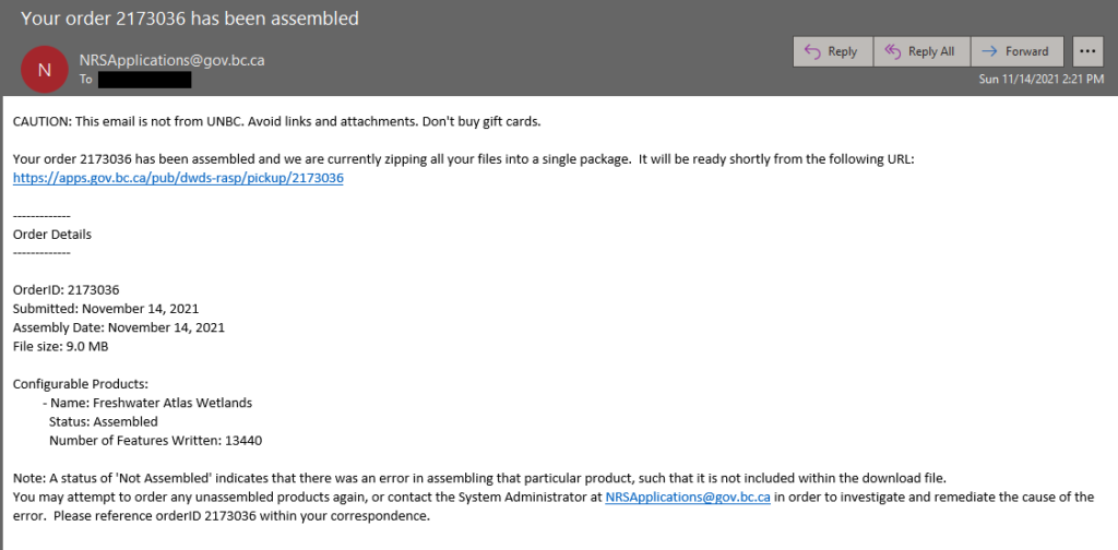
Finally, type in the email address where you want DataBC to send your download link, and submit your order.

In a couple of minutes, you’ll receive two emails. One as a sort of receipt, and the other with your download link:

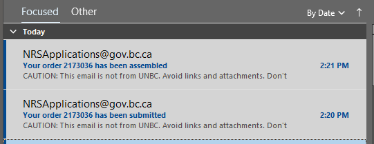
Click on the link in the email, and your file download will begin. Extract the zipped file, and you should be good to go.

Next week…

Next week, we’ll go over saving multiple layers to a single Geopackage, which is a really nice way to bundle up your project for submission. For now, go ahead and get started on your projects!