Lab 07 – Mixed Data Formats

Using data from mobile phones, raster and vector data

We are going to look at some GPX data (the type that comes off your phone when collecting tracks and waypoints using GPSLogger, OpenGPX, and other methods (like GPS units). We will then take it into QGIS and ArcPro to do some analysis with it.

GPX Files

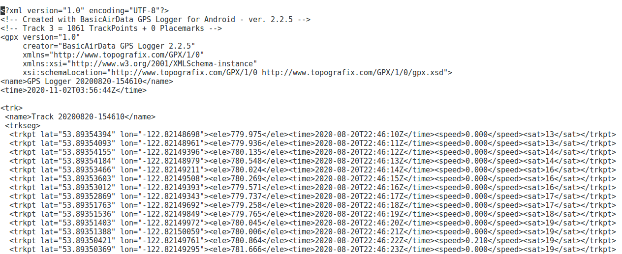
A GPX file is the standard file for sharing information from devices (GPS/GNSS device) or mobile apps. It is an XML based file format that records a point location at a certain interval – time based or distance based. Here is an example of the GPX file we will be playing with this week.

The top of the file:
Click the image for a larger view

End of the file:

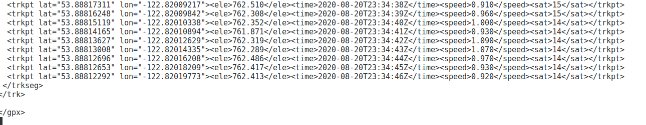
As you can see the text in the file (much like we saw with the Postalcode text file) will create a system of points than can be joined to create lines.

Part 1:

Adding a GPX file to software

We are at the point where we want to use the software that makes life the easiest. ArcPro can read GPX files, but you need to use a processing tool – QGIS just opens the file (so we will use QGIS this week).

Steps:

• Open QGIS and add in the GPX files in L:\GEOG204\lab7 folder (scott_roger_explore.gpx and scott_roger_explore_poly.gpx)
• Select the track points and tracks only for each dataset
• You will end up with two sets of data with almost the same names in the TOC, but you can tell them apart by the completeness of the track lines and the extra point in the “poly” file
• Add in a web map background to see where the data is located – the ESRI Topo layer provides a nice view of the terrain

Investigate the data

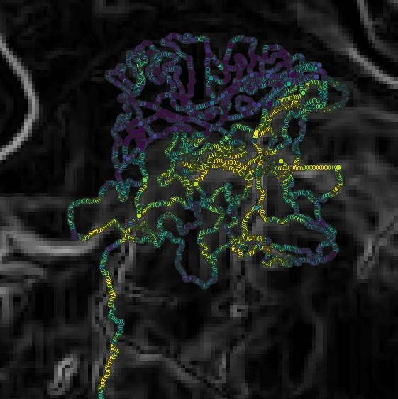
You can see from looking at the data, we lost satellite reception often in our walk, but there are plenty of places to check out data under the track points. You can also see there are elevation values collected from the GNSS app in Scott’s phone. Lets compare it with a DEM from 2018 LiDAR data.

DEM data with point data

Sample raster data

Consider what we are doing by sampling raster data: wherever there is a point in the vector layer, the corresponding raster value will be saved into the vector layer’s attribute table.

• Add in the scott_roger_explore_dem layers into the project (Drag and Drop or Layer –> add Raster Layer)
• Find the sample raster values in the processing toolbox
• Fill out the panel appropriately – it does not matter which point layer you use as they are the same data

Input Layer: track points

Raster Layer: scott_roger_explore_dem

Output column prefix: SAMPLE_DEM

• Look at the new layer’s attribute table and note the column name that was added (SAMPLE_DEM1)

Do some math

• Open the attribute table of the new layer
• Use the Field Calculator to create a new column (dem_diff) that computes the difference between the GPX elevation (ele) and the LiDAR DEM data (SAMPLE_DEM1)
• Style the layer to see the differences: if you are illustrating a range of values, what symbolization style would it make sense to use (single symbol, categorized, graduated, etc.)?

What kind of range do you get in elevation difference? Quite the error in elevation values from mobile phone GNSS data collectors!

• Style the sampled layer with graduated color, 2 classes with range value from the lowest to 0 and 0 to the highest in sample_dem

Clean up your GPX data

• Have a look at the attribute table of your sampled and calculated layer, and take note of all the fields that are not useful to you
• Right click on the sampled and calculated layer –> properties
• Select the Fields tab in the panel
• Ensure the layer is in edit mode (toggle the yellow pencil icon)
• Select all the fields you are not interested in keeping (probably most of them)
• Hit the delete field button to remove the fields
• Turn off the edit mode – turn off the pencil
• Close the properties panel

Export as a new file type

Export the data in the usual fashion, BUT, we’re going to export into new format, a Geopackage:

• Export as a GEOPACKAGE
• Export the data in the local UTM projection (EPSG: 26910)
• Call the layer whatever you wish (e.g. my_point_demdiff.gpkg)

Copy the Styling from the Original Dataset

• Right click original layer > Styles > Copy Style > All Style Categories OR Symbology
• Right Click the new Geopackage (my_point_demdiff.gpkg) > Styles > Paste Style > All Style Categories OR Symbology

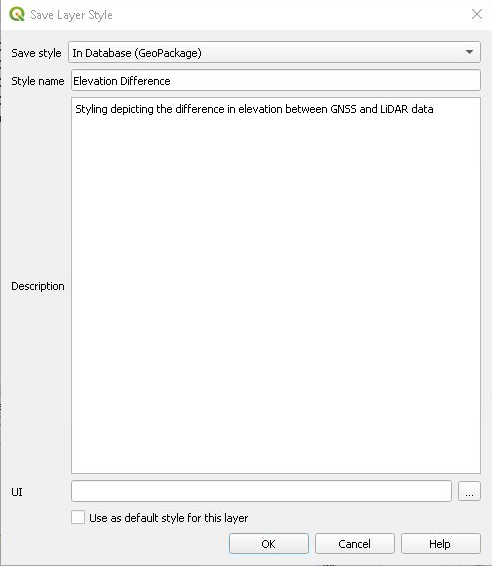
Save the New Styling to Your Geopackage

• Right click on your geopackage layer > Properties > Symbology
• In the bottom left corner of the Symbology tab, click Style > Save Style
• Change Save Style to In Database (GeoPackage) –> give the style a name and description

Part 2:

Create a polygon and get some statistics

Using the GPX layer that has the potential to be made into a polygon (scott_roger_explore_poly.gpx), create a polygon layer using methods we’ve used in previous labs.

Once that is completed, sample under the polygon to get elevation and slope data.

Here are some suggested steps:

• Create a polygon from the track layer with the Line to Polygon tool
• Run the Fix Geometries tool on your new polygon layer
• Create a slope layer from the DEM layer with Slope tool
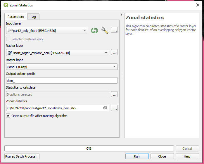
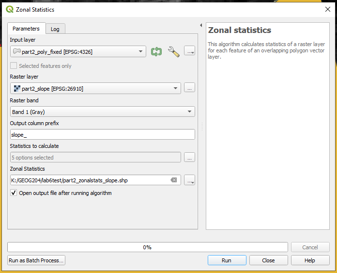
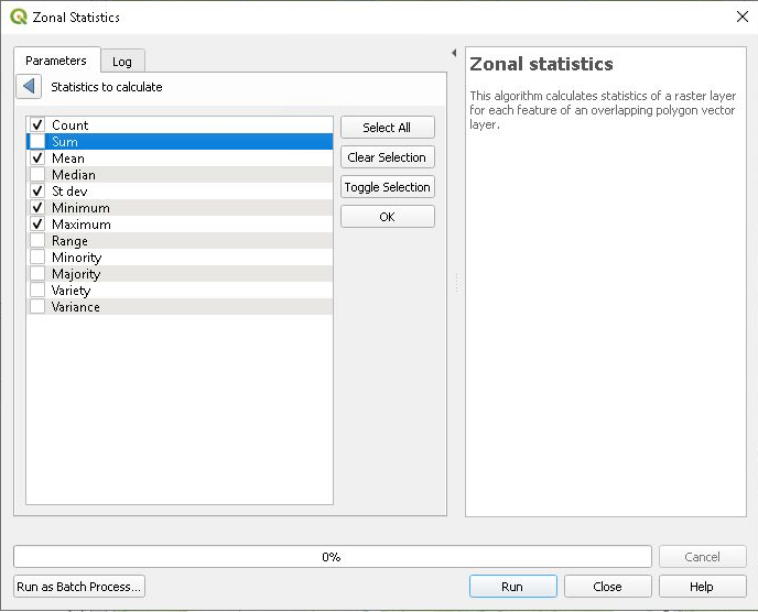
• Sample under the polygon using the zonal statistics tool with the following parameters:
  • include count, min, max, standard deviation, mean
  • Sample both the DEM layer and the Slope layer: use the prefix “dem_” for the DEM sampling and “slope_” for the slope layer
• Check out the sample images below

Clean up the unnecessary attribute fields like we did earlier and save this as a second geopackage (no need to worry about styling)

Check against the track points

Check the elevation differences you sampled with the point data (where Scott and Roger walked)

• Find the Basic Statistics for fields tool
• Run this on the geopackage dataset for the sampled points (from Part 1) using the LiDAR elevation values (the field called something like SAMPLE_DEM1) as the “Field to calculate statistics on”
• Click run, but don’t close the window yet: the report will be generated in the log pane
• How do the min, max and mean values compare here (from the point layer) to those calculated in the polygon layer using the zonal statistics tool and the DEM layer? You may wish to jot them down somewhere since you’ll have to navigate to another window.
• If you mistakenly close the window too soon, you can find the results from the tool you just ran in the Results Viewer pane by double clicking on Statistics:

Let’s review what we just did:

In Part 1, we sampled elevation data against the track points from the GPX data, then calculated the statistics for those sampled data just now. In the attribute table, each point had an entry and had its elevation saved after we sampled it. To see the statistics of the elevation data stored in the attribute table, we ran Basic Statistics for Fields, and created a separate output with the statistics.

In Part 2, we calculated the elevation statistics for the area covered by the polygon that used Scott and Roger’s hike as the perimeter. The summary statistics that we requested were then saved to their own fields in the resulting attribute table of the new polygon output.

Save your project

Assignment 7 – 5% due next week:

• Open a new project and save it as assignment7
• Add trails and DEM file 93g-dem25m-utm10.asc from L:\geog204\lab7

Clean up the trails

• You can see all the trails except Ferguson Lake (north of the DEM) fit on the DEM. Remove this trail loop by:

• With Select feature tool to draw a Rectangle to all trails except the loop for Ferguson Lake.
• Right-click trails > Export > Save Selected Features As
  • Format: GeoPackage
  • File Name: A7
  • Layer name: my_trails
• Check if it worked by Zooming to Layer of your edited Trail layer – it should now exclude the Ferguson Lake trail loop, and all of your trail layer should fall within the DEM you just imported
• Turn off the original trails layer

We want to see the difference between using a couple of tools for determining how difficult a trail may be to walk compared to checking points along a line sampled against a slope layer. You will carry out this check using the following steps.

1. Use the Drape tool on your trail layer to get elevation values (“Z” values) from the DEM layer we just imported to create a 3D line layer (0.5 mark). Check out the description for each of these tools on the right hand side of the tool window to learn more about what each tool does.
2. Use the Climb Along Line tool on the output to generate some climbing attributes for this layer (0.5 mark)
3. Create a new line layer by using the Densify by Interval tool with a 20 meter spacing using your trail layer as input (0.5 mark)
4. Create a new point layer by extracting these new vertices created from the densified line using the Extract Vertices tool (0.5 mark)
5. Create a slope layer from the DEM (0.5 mark)
6. Sample the new point layer against the slope layer (0.5 mark)
7. Style the climb layer (use the ‘descent’ field) and the sampled point layer (use the SAMPLE_1 field) as graduated using the same colour scheme with the same number of classes for both layers in order to compare them visually (1 mark: 1 for each layer’s styling, shown in your screenshots)
8. For your write-up, describe the steps you took to get your results (1 mark). Use the tool descriptions to help you describe what you are doing in each step. Feel free to include screenshots of the different steps. Do include screenshots of your two resultant layers (one line layer, one point layer) against the slope layer you created as a base layer.
9. Save everything in one WORD file as lastname_firstname_geog204_A7 and submit to your TA

Below is an example of this type of output. It’s a zoomed in portion of the trails, but for the assignment we would like to see all of the Prince George trails (excluding Ferguson Lake). Make sure to include your Layers panel in the screenshot so we can see the classes you sorted by