Lab 02 – Creating Data

Making use of text data, tables and digitizing

Learning objectives:

• Importing and displaying coordinates from a .csv (text) file
• Joining tabular data to spatial data
• Saving data to different formats
• Creating lines from points and polygons from lines
• Creating new shapefiles
• Digitizing data

Taking tabular data and bringing it into QGIS

Data Management

Make a folder for today’s lab to save all your data into (i.e. lab2 in your geog204 folder). Once it is created, copy the following data from the L:\GEOG204\labs\lab2 folder:

• postal.txt
• theftsfrom.csv

Cleaning the data

Right click on the postal.txt file and open with Notepad in Windows.

Take a look at the data and see if you can figure out what is going on.

• Clean off the metadata, set up the column names to be Postal, Lat and Lon and save the file in your folder.
• What are the commas used for?

Open the file theftsfrom.csv in both in a text editor and in a spreadsheet program (e.g. Excel or LibreOffice Calc).

• Do you understand how the data is put together? Do the commas from the postal code dataset make more sense?
• What type of data is being recorded?

Bringing text data with and without coordinates into QGIS

Open a new blank project in QGIS. We are familiar with shapefiles and we should know how many files make up a shapefile, but the files you have looked at today are simple text data. Data like this can be loaded in such a way to create point features from plain text.

Open the postal code data by:

• Layer –> Add Layer –> Add Delimited Text Layer –> choose your postal code file you cleaned above
• Set up the import panel to make use of the x, y coordinate in the file
• What are the x and y coordinates? The image below should help you out.

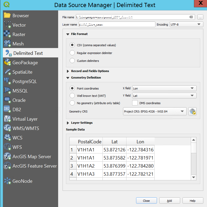
What does this data show us?

You can follow a similar process to add the thefts data, but since there are no coordinates to reference each features’ location in space, it is just a table – select the option that tells QGIS to not consider the file a spatial layer (no geometry).

Base map – and plugins

Plugins

We have looked at QGIS a fair bit it the last two labs, but we have yet to look at one of the great features of the software – Plugins

QGIS allows people to write their own plugins, which adds functionality to the software. Use the menu along the top of QGIS window to Manage and Install Plugins.

• Go to Plugin->Manage and Install Plugins
• Click the settings tab and turn on all the check boxes so you can see experimental plugins
• Go back to the All tab and search for the QuickMapServices plugin and then Install Plugin

Plugins sometimes get added to odd places, but you can find this one on Web Menu –> QuickMapServices

Once you are there add the contribution pack to the plugin by
settings –> more services –> get contributed pack –> save

We have two data sets in our TOC (table of contents). We can add a background map to get some reference using the QuickMapServices plugin. If you go to the plugin under web, choose a background that you like (i.e. OSM–> OSM standard or ESRI–> ESRI Topo)

Bringing the datasets together – they are much more useful this way

We want to be able to see where each vehicle from the theftsfrom file was stolen, but that file has no geometry with it. What we do have is points for each postal code. Is there something in common that will allow us to join them together?

Open the attribute table for both layers so you are familiar with the attributes that are listed.

Joining Tables in QGIS

Right click on the thefts layer–> properties –> joins tab

• Add a join (plus button)
• Select the Join field (Postal)
• Set Target field to Postal Code
• Click OK

Open the attribute table and see the difference – there should be lat/long values listed

Now that the table is joined – save the theftsfrom layer as a CSV type and bring it back in as a spatial layer.

Right click thefts –> Export –> Save Features As

• Format Comma Separated Value
• Choose a name and location

Even though it adds it in automatically after you save it, it doesn’t recognize the geometry unless you add it back in. Since it now has coordinates in the attribute table, you can add it as a CSV with coordinates.

Now save both the postal layer and the thefts point layers as shapefiles in your folder.

Reviewing your data and your thought process

It is always important to take a critical look at your datasets and outputs. Look at the distribution of your points, does it make sense when you compare the postal codes to the thefts? Does it matter that there are more thefts than postal codes?

Question 1 (1 mark – answer all parts of the question for the full mark): Why isn’t the postal code a unique identifier in this thefts shapefile? Does each postal code have a theft? Is the theft point the ACTUAL location where the theft happened, what is your reasoning behind this? What about thefts that happened in the same postal code – how do they get displayed?

A quick way to add Unique Identifiers in QGIS

Lists of attributes like this should have a unique identifier. It is a good practice to create unique IDs. Often we are working in the geometries of a layer or features, but we also spend much of our time altering the attributes of each layer. In this case we are cleaning up the data through its attributes by adding a unique ID.

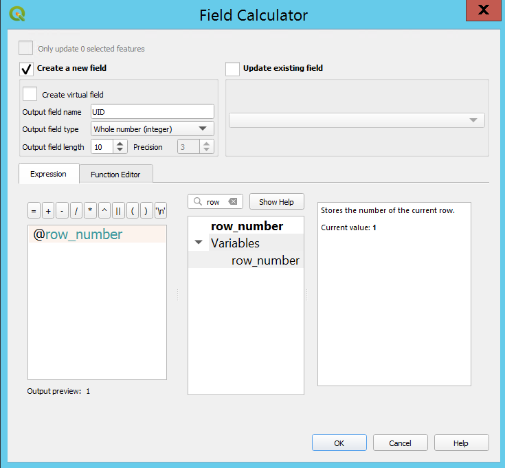
Open the attribute table –> open field calculator –> new field. Set the field as the following:

Output field name: UID

Output field type: Integer

Enter the “@row_number” function in the expression panel –> Click OK

Creating lines from text files

Line generate files

We just created a point feature type layer. This file did not have a unique ID for each location associated with each row’s x,y coordinates, but rather postal codes (that are not necessarily unique) so we assigned it a unique ID. The data we started with were stored in a text format using delimiter such as commas and is often called a generate file–we were generating a point layer (one feature per row of text). This concept can be extended to creating lines and polygons from text using the Simple Features Model.

It is possible to create lines by personally digitizing (connecting) points, but it is also possible to generate a line by connecting points (or vertices).

Generate file for lines:

12
0.5121700E+06 0.5971884E+07
0.5121580E+06 0.5971892E+07
0.5121380E+06 0.5971892E+07
0.5121310E+06 0.5971972E+07
0.5121270E+06 0.5972053E+07
0.5121840E+06 0.5972065E+07
0.5122610E+06 0.5972076E+07
0.5122700E+06 0.5972009E+07
0.5122740E+06 0.5971961E+07
0.5122420E+06 0.5971934E+07
0.5122440E+06 0.5971925E+07
0.5122720E+06 0.5971930E+07
0.5122770E+06 0.5971895E+07
0.5122720E+06 0.5971894E+07
0.5122250E+06 0.5971885E+07
0.5121700E+06 0.5971884E+07
END
…

9
0.5118040E+06 0.5971068E+07
0.5118470E+06 0.5971000E+07
0.5118070E+06 0.5970966E+07
0.5117430E+06 0.5970930E+07
0.5117200E+06 0.5970950E+07
0.5117090E+06 0.5970949E+07
0.5116780E+06 0.5970993E+07
0.5117120E+06 0.5971018E+07
0.5117230E+06 0.5971014E+07

0.5118040E+06 0.5971068E+07
END
END

This file type is the same as a file for points but for lines. The first number indicates the start of each individual line by giving it an unique ID (“9″ and “12″ are the unique IDs for the two lines). The rows of numbers after the ID represent x,y coordinates (in this case UTM coordinates – we will learn about this later) and the END statement defines the termination of each line as well as the completion of the layer (end of the field). These numbers can be brought into GIS software to make shapes (the campus buildings actually). Instead of generating these features we are going to use bear point data to create a line that expresses the movement of a bear.

Question 2 (1 mark – answer all parts of the question for the full mark): Last lecture we learned what the start and end points on a line are called as well as the points along the line. What feature types can be created for the file above (the generate file)? Explain your reasoning using the terms we learned in lecture.

Making lines from points

Load the bears95 file from this week’s lab folder on the L: drive. You can also load the roads shape file from this week’s lab folder.

Make sure you have your Processing toolbox panel visible.

First thing you should always do is explore the dataset, understand what the attributes are. If we inspect some of the points in the bear layer we may guess as to the probability of there being one bear in several areas over a period of time. Pick out several points of interest to build a line from.

• Add bears95 and roads layers – as shapefiles
• zoom to an area of interest
• use the select tool (Select menu –> select by rectangle)
• Search for the tool “Points to Path” in the toolbox panel
• order by “date_path”
• group by “Activity_c”

You can play around with grouping and ordering the creation of the line as you see fit. You could even try to group by DATE and order by Date_path. Too bad we do not have the time of day the data was collected.

Make sure you have saved you output as a shapefile – otherwise you could lose your work.

You should also save your project (Project –> save project). As the semester moves along, you will realise that saving often is very important. Often students will save may versions (e.g. lab1a, lab1b…) that they loop through in order to take a step back if you did something crazy in your project.

What is the difference between saving your project and saving layers as shapefiles?

Digitizing – Points to Lines to Polygons

Start a new project.

As the use of GIS and related fields have become more commonplace, there has been a great amount of data created or collected. For instance the road layer we are using could have come from municipal CAD drawings or digitized directly using GIS. This means that at one time, all old data had to be digitized (drawn using digital means – a computer) by applying similar techniques as we are about to use.

Steps for digitizing

Using the bear95 layer we will trace some points approximating where a bear’s (or several bears’) cruising ground is. We want this new layer to be clean, so we need to apply the concepts of threshold and snapping.

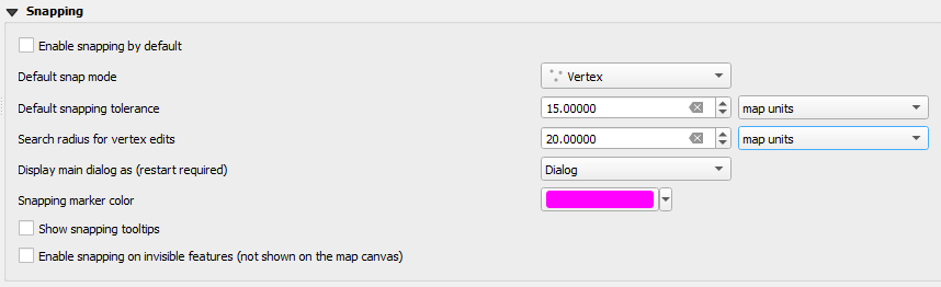
• Go to settings –> options –> digitizing
  • In the snapping section:
  • Set default snapping tolerance to 15 meters (map units)
  • Set search radius for vertex edits to 20 meters (map units)

• Add a new “line” shape file layer (layer –> Create layer –> New shapefile layer)
• Check the projection to be UTM 10 (26910)
• Start editing by applying the “yellow pencil” (can be done by right clicking the layer or hitting the menu button)
• Add the snapping toolbar from Project->Snapping Option. You can pick the layers to snap to (Advanced Configuration –> Open Snapping Options) and customize the snapping options:

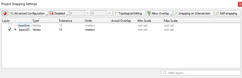
• Draw some lines – three or four that connect (try to snap to bear location points – look for the red target), and three or four that don’t connect
• Save your edits to your new layer

Turn them into polygons – Two Ways

• Under the Vector menu use the “lines to polygon” function to create polygons.
• Repeat the polygon building by using the polygonize tool (It can be found in the toolbox you used earlier)

Thinking about the difference between these 2 ways of making polygons

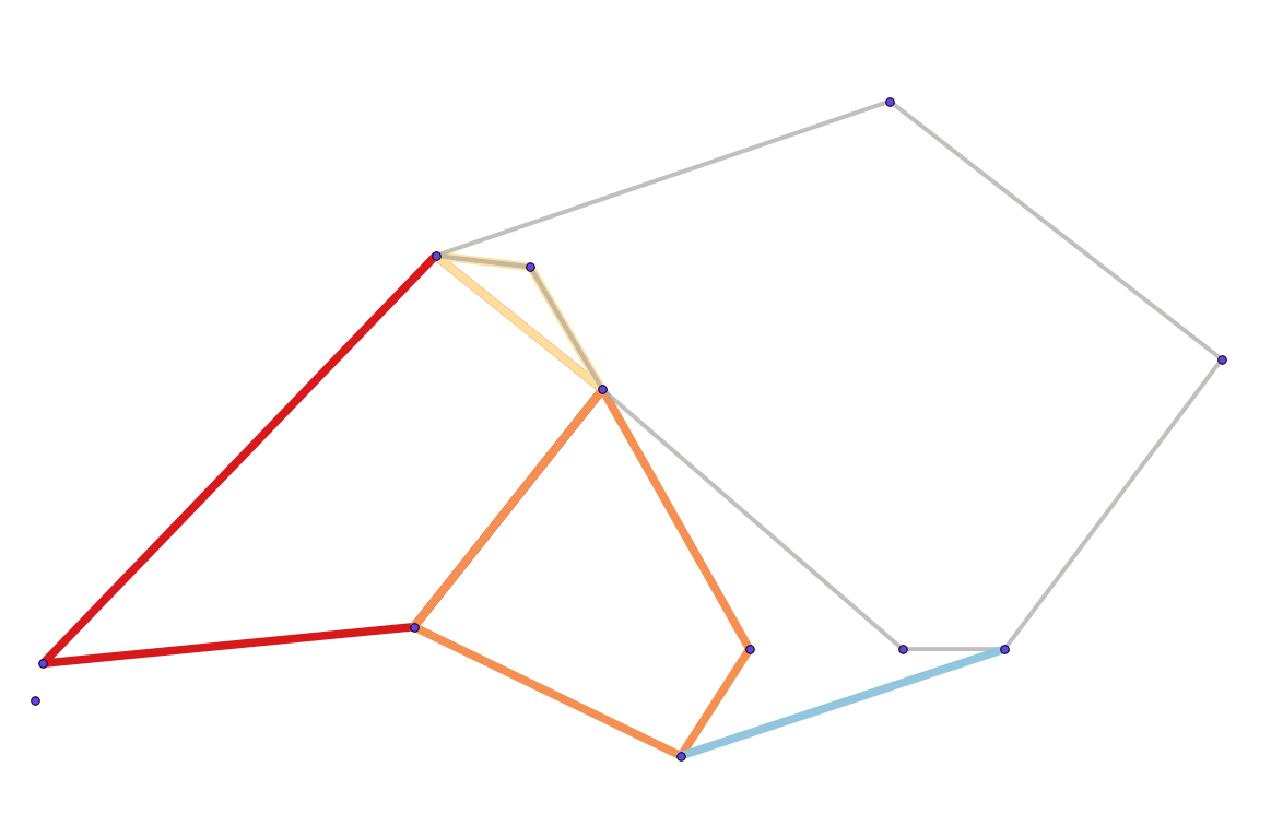The first illustrates the lines that were digitized from following the point layers – (i.e. turning on the snapping options to make use of the bear point layer below our line that is digitized).

The lines were drawn in the following order:

1. red (it is underneath the lines the yellow and orange lines share with it)
2. yellow (it has common lines with red and grey)
3. orange (sharing with red)
4. grey (sharing with yellow)
5. blue (is shares with no other lines and has only two vertices)

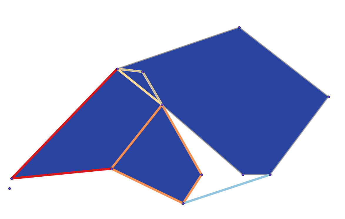
The second illustrates the polygons created using the Polygonize Tool.

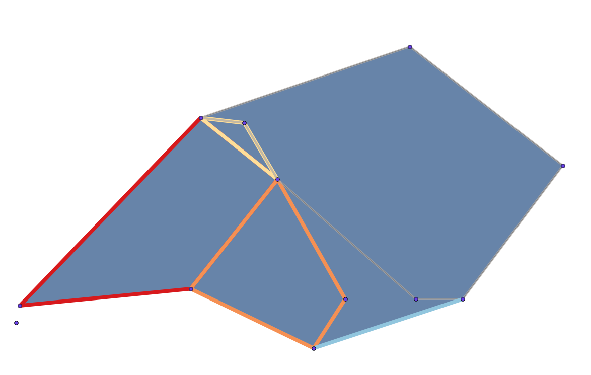
The third is the polygons created using the “lines to polygons” feature standard under the Vector menu.

Question 3 (1 mark – answer all parts of the question for the full mark): Try to explain why the two polygon layers are different. Can you determine the process used to create the polygon features?

Create polygons directly

Using the skills we just learned, create a new polygon shapefile and hand digitize an area that you would want to investigate further – like an area of interest that you would focus the rest of your work on.

• Create a new “polygon” shapefile layer
• Activate editing of that layer
• Go to settings –> snapping options
  • Click to activate the bears95 and your new polygon layer
  • Set the snapping tolerances to 20 map units
  • Set to both “Vertex and line” in the snapping toolbar
• Draw some polygons
  • Draw features without them touching (0.25 marks)
  • Draw features that are clean and touch (0.25 marks)
  • Draw features that overlap (0.25 marks)
  • Draw some holes in some feature (you will have to find your advanced editing tool bar) (0.25 marks)
• Add vertices to features
• Move vertices within features
• Save your edits

Question 4 (1 mark – see distribution above): (take a screenshot for each step above)

Adding your KMZ/KML file to QGIS

Open up a new project in QGIS and add KML file from the L:\ drive (e.g. PG_photos.kml), or you can load a KMZ file from your K:\ drive) if you have any.

Once that is loaded, use the QuickMapServices plugin to add a webmap base layer below the points to give geographical reference to your data.

Question 5 (1 mark – see distribution below): Include a screenshot of your KML/KMZ file (0.5 mark) with the base map (0.5 marks) in your write-up. You can use the snipping tool (or something similar on you own computer).

Assignment #2 – 5% due in two weeks (the week of Oct.2)

• Save the answers for the questions 1, 2, 3, 4, 5 in a Word document labelled as lastname_firstname_geog204_A2 (Note: Do NOT forget your name and studentID in WORD file). Send it to your TA