In this course we will use both QGIS, a free and open source software package that is developed using open standards, and ArcGIS by ESRI, the most popular desktop GIS software globally. With the software being Open Source, you can download QGIS on your personal computer (even for those non-Open Source Operating systems).
The theory and methods you learn in this course can be applied in QGIS, ArcGIS and other GIS software
This introductory lab is meant to walk you through:
– Working with project files in QGIS
– Accessing spatial data
– Downloading Open Data
– The basic interface features of QGIS
– Working/understanding spatial data layers and attribute tables
– Styling your spatial data
– Composing a simple map
Locating data for the lab:
Data used in the GIS Lab
The first data set we are going to use is located in the labs folder on our GIS server (L:\GEOG204). This is where you will find all the spatial data used for for the courses as well as other data used for projects.
Understanding where data is and how to manage your own spatial data:
Before we start QGIS, lets ensure we understand how were are actually managing the data we will be using for Geog204.
- Open a file browser and check if you have two network drive labelled as K and L. The K drive is your home directory with full access, the L drive is read only with all course data and other spatial data.
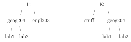
- Open the file browser, create a new folder in your K: drive called geog204. You will find it easier to create folders (also called directories) with no spaces in the name (a good practice for outside the GIS Lab as well). Inside the geog204 folder, create a sub folder called lab1. This is where we will be putting files for our lab this week. Below you can see a sketch made using a keyboard that shows the tree (upside down) perspective of how files and folders managed. It is always a good idea to find out where files are stored on a computer (not just accepting the default locations such as “Documents” or “Photos”.
Getting data from the lab folder:
Spatial data comes in a variety of types and formats. It comes in all sizes and without proper management, looking for spatial data can become a real nightmare. Using the file browser on the desktop of the computer navigate to L:\geog204\lab1. You will notice the files that are used in QGIS.
If you set your browser to present the contents of the folder in a list (or details) view, you can see that there are files with the same name but different extensions. You can look up what the different file extensions are used for (what files are associated with specific software or uses) by going to fileinfo.com. This does not really work for the files we have in the folder though. These files represent layers that will be added to QGIS in the form of a “shapefile”.
Question 1 (1 mark):
How many files represent each layer we are going to use in the lab today (i.e how many files for “pg_rivers”)? These files represent “shapefiles,” and unlike software such as MS Word, more than one file is required for a shapefile to be used in GIS software. Determine which of these files are mandatory for use in software (HINT: use Wikipedia).
You may have also noticed there is a file with the extension .qgs. This is a QGIS project extension. We will be using it in the next section.
Opening QGIS and getting started:
To open QGIS you click on the ‘Start’ button on your screen. Now type qgis you should be able to see the QGIS Desktop program – open it.
In order to give you the opportunity to more easily explore QGIS, we have provided a project file. As mentioned above, project files end with .qgs and contain the information necessary in saving and reloading your work. You can find your project file options under the Project tab. Go ahead and open up the Lab1.qgs file you navigated to above.
- Project –> Open –> navigate to L:\geog204\lab1 –> Open lab1.qgs.
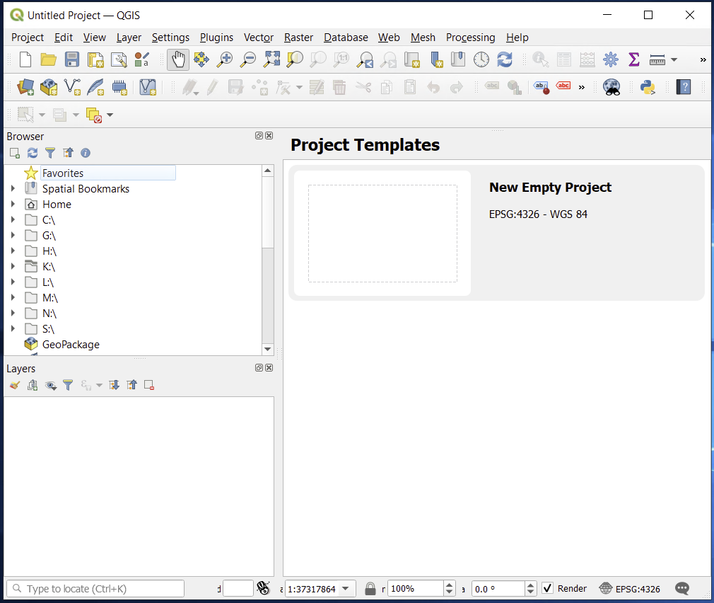
You should have some Prince George relevant data on your screen! You may also notice that your screen is slightly different than the one shown here (click on the image for a larger view). This is because many of the windows and shortcuts to tools can be added and removed from the main screen of QGIS. You can customize QGIS to make your life easier.
Let’s first save this project file to your local K: drive so you will have full access to the file.
- Click Project –> Save As and navigate to K:\geog204\lab1 and save it as my_lab1.qgs
Panels and toolboxes:
You can add and remove panels by right clicking within the empty gray space along the top section of the QGIS window. Let’s just start with at least the Browser Panel and the Layers Panel enabled. They should be on by default, but you can add others if you wish. Other useful panels are:
– Processing Toolbox
– Log Messages Panel
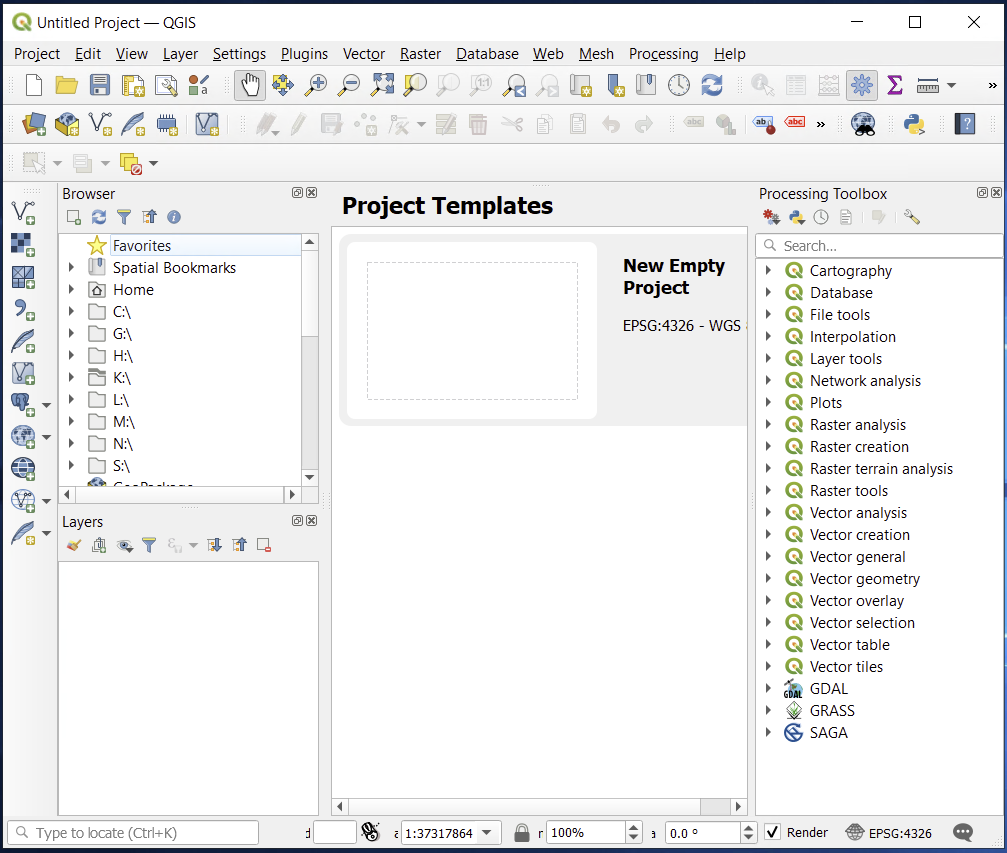
In addition to adding and removing panels, you can also move them around the screen, providing the opportunity to customize the user interface to reflect the features you want quick and easy access to.
Below is an example of customizing your qgis session:
Browser Panel
Check out the Browser Panel and compare it to the files that exist in the folder by using the windows file browser. What do you notice about the number of files in the QGIS Browser compared to the File Browser?
See if you can load the pg_rivers into the QGIS project. Style the layer accordingly.
Panning and Zooming:
Let’s try to provide a screenshot of a park area within Prince George. This screenshot must contain the entire area of the park. As you will find out with GIS there are often many ways you can accomplish tasks such as this one.
Some of the tools you will/could use to accomplish this are:
– The Pan tool (the white hand icon that is usually the default tool when you turn QGIS on) allows you to move around the map content screen (or often called the map canvas).
– Icons that have magnifying glasses are usually associated with a zoom feature. There are many different zoom features, and ways to access them. The scroll button on your mouse will zoom in and out the same as the zoom + and zoom – tool. Take some time to try out what these different zoom features do.
Data Layers:
Inside the ‘Layers’ panel (often called the Table of Contents), you should see a list of layers that were loaded when the project file was opened. Do you notice the layers stack up for maximum visibility? Area layers (polygon layers) are at the bottom of the list, with line layers on top of them and points finishing the map off. Ensure the Trees and Park and Open Spaces layers are turned on by clicking on the check box beside the layers in the layer panel.
You can change the order of layers by dragging them up and down in the Layers panel list. The way these layers are displayed is based on the order they appear in the Layers panel. This means a layer that is turned on and is on the top of the list is drawn on top of the enabled layers that fall below it, in a stacking effect.
Layer Properties:
By right clicking on a layer within the Layers panel, a list of options appears. Open the Properties for a layer. Properties are useful for but not limited to the following: general information about the layer, labels, metadata, and styling.
Under the Information tab of Properties, you have easy access to the name of the layer, the name QGIS is displaying for this layer (it will be different than the name of the layer if you have renamed a layer in QGIS), the location of the layer on your hard drive, and the Coordinate Reference System of the layer.
The Metadata tab is essentially the citation information of the layer. You will likely notice that this section is often left blank, though ideally it would always be filled out correctly.
The Symbology tab allows you to change the appearance of layers on the map. You will need to use this for the final output of this lab, a map.
This is by no means a complete overview of all the tabs or even what individual tabs can do. Instead this is a quick overview of some of the basics you need for this lab.
Attribute Tables:
Spatial layers are more than just lines drawn on the screen, they also contain information for each feature in the layer (hence the “I” for Information in GIS). For example the trees layer has the name of the type of tree for each point on the map canvas, where each point represents a tree location. You can open the Attribute Table of a layer by right clicking on it within the Layers panel. You will notice that the attributes for the features in the layer are presented in the same manner as a spreadsheet (such as those used in Excel).
Highlight a layer in the layer panel (perhaps the parks layer) by clicking on it once – the layer should now have a blue band over it. This makes it an “active layer”. We can then select features in this layer. Open the attribute table for this layer as well.
You can select features in the map by using the “Select Features” tool. Hover your mouse over the tool icons until you find the “select features by area or single click” tool
Activate Select_Features by clicking on it. Once the tool is active, select a feature in the layer. Check the attribute table once a feature is selected – you will notice that a row in the table is also selected.
Do the reverse by selecting a row in the table and use the attribute table tools to zoom to the feature selected.
Question 2 (1 mark):
What is the name of the Park that one of the three Siberian Elm trees (CommonName) in Prince George is in? Once you have selected the tree within the park, take a screenshot of the selected tree and a portion of the park.
Creating a map using Layout Manager:
Map essentials
This course is not designed to spend a significant amount of time on teaching the art of making good maps, as this is covered in GEOG 205 – Cartography and Geomatics. However, it is important to at least mention some of the basic components of a map that you will be expected to include in all of the maps you hand in for this course. You will generally need to have: a title for your map, your name on the map, a legend, a north arrow, a scale bar, and, when appropriate, a description.
Layout Manager is the tool you use to create a map, while the window you have been using to explore the data up until this point is more of a data view window. To open up Layout Manager, find it under the Project menu, and give your map a file name. Most of the tools you will need to use to make your map are found under the Layout tab.
To add data you have prepared in your projects data view window, use the Add Map tool. You are now able to create an area (drag out) the size you want to be filled with your map content. You will want to consider the space needed for the title, legend, north arrow, scale bar, your name, and any other pertinent information. You can resize and move this at any point in the map making process.
After you have added data, you may notice that the data view and map view you just added don’t look exactly the same. You will probably have to pan around and change the resolution to work in the Print Composer, which can be done using the Move Content tool. The actual Zoom buttons within Print Composer are a bit misleading, instead of zooming the map panel content it actually zooms the entire Print Composer window. Using the scroll wheel on the mouse when Move Content is enabled is an easy way to zoom in or out.
Title: To add a title you will create a Label, which will appear in the Item list. In the Item Properties tab of this label you can add the title text. If you think the font is not the ideal size, this can be changed in the Font menu. You can add your name and a brief description to the map using this same procedure.
North Arrow: Use the Add Picture tool and pick a size and location for the north arrow. Similar to creating a title, use the Item Properties and expand the Search Directories options, where you will see previews of the pre-loaded images provided in QGIS. Pick a north arrow you like, and if the north arrow doesn’t appear, you may have to manually adjust the styling options for it. To do this, open the SVG Parameters found under Search Directories. It is also possible to create your own images or find other images and use them as well (but you are by no means required to!).
Scale bar: By now you are familiar with the general process of adding additional map elements, so add a scale bar. It is important to make sure that the units being displayed on the scale bar are appropriate to the context of the map you are creating. For instance, it would not be appropriate to have a map with a scale bar measured in miles when the map is for Prince George (Canada).
Locking layers in place: At this point, you have enough separate elements in your map that you may have run into some frustration by having something positioned and sized perfectly only to accidentally move or resize it. Any of the items you’ve added to the map can be locked in place (which also locks their styling). This option can be found in the Item Properties, and can be disabled if you need to make any changes later.
Legends: If your legend has auto-populated all the layers from the data view window, and you want to change this – disable the Auto Update feature in the legend’s Item Properties menu. When Auto Update is disabled, you can reorder or remove layers from the legend. You only want the legend to show the layers you actually have in the final version of your map, so take a moment to verify everything is in order. You can also change the background colour and many other design features in the Legend item features.
Question 3: Export your map (1 mark)
Create an export of your map – it does not have to be fancy looking – by using the export function in the composer. You can export the map in a few formats, but for the sake of bringing the map into software such as MS Word, we will export the the map as an image. Layout –> Export as Image –> choose the file (ensure it is a PNG or JPG).
Downloading and adding data to your project:
We downloaded the data layers for this project from Open Data Prince George (the city of Prince George data sharing site) at http://data-cityofpg.opendata.arcgis.com/
Visit the site and perform the following steps
– download at least one shapefile to your geog204/lab1 folder
– the file will come down as a compressed zip file
– locate the file in your folder and decompress the contents of the file (right click –> Open with Archive Manager –> extract it to the folder)
– open the data layer into QGIS (Layer –> Add Layer –> Add Vector Layer –> navigate to the folder and select your layer
– style the layer accordingly
Question 4 (2 marks)
Follow the steps above to add the Incorporation Boundary layer to your project. Once you have it loaded, perform the following steps to provide another screenshot of your results:
– Style this layer by using the “categorized” method using the attribute column for year of incorporation (Incoorporat)
– Place the existing layers in an order for proper viewing
– Colour the one feature in your new layer red that matches the criteria described next
– Take a screen shot and include it in your write up
There is one more Siberian Elm tree located in the Millar Addition of Prince George. Read the Wikipedia article on the Millar Addition and determine which year this area (part of a larger incorporation boundary feature) was incorporated (the closest year). The feature that includes this year is the feature to colour red.
Do any of the the Siberian Elm trees in the pg_tree layer fall within the Millar Addition?
Finish up
After your screenshots and exports are saved and you have begun to write up your lab, save this project to your lab1 folder (maybe call it something simple like – lab1). You then can close QGIS and log out.
Assignment #1 – 5%
- Create a title page with course name, student ID, student name, and your lab section. A title page should be included in each of following assignment.
- Answer the four questions posed throughout the lab instructions.
- Insert your screenshots as images in the file.
- Save everything in a single WORD file as Lastname_Firstname_GEOG204_A1 (Please name your assignment properly)
- Submit the WORD file to your lab instructor through Moodle.
Late assignments will be docked 5% per week, but please get in touch with your TA if you have a problem with a deadline.