In today’s lab we will be logging into the various accounts we will be using, looking at how the file server works, and getting to know ArcGIS Pro, the primary software we will be using this semester.
Housekeeping
During Labs, you are encouraged to ask questions and interact with the material. As always, if you have a question, it is likely that there are others with the same question, so please speak up.
We also ask the following in the GIS Lab:
- Please do not unplug anything already plugged in in the lab. If you need to plug in personal devices, there are some plugs located along the outside walls of the room, or the odd empty plug available in the center power bars.
- Do not turn off computers when you are done using them, as all the machines need to be on to receive regular system updates.
- Do sign out of your lab computer every time you are done in the lab. The same goes for every time you use Osmotar (more details below).
Your Workstation
This lab is equipped with powerful workstations running GIS software. However, one quirk we would like to cover is that you have two monitors. When we upgraded the lab computers, we opted to keep the old monitors for viewing web pages and word processing. One of your monitors is 13 years old, with varying degrees of fading affecting colour reproduction, has HD resolution and 8-bit colour. The other monitor is a year old, and able to display 10-bit colour, Ultra HD resolution, and is calibrated for constant display. This consistent display helps when judging colour choices. You should always be using ArcGIS on the higher resolution screen.
*On this topic, we recognize that colour blindness is relatively common and affects how we perceive the quality of colour choices. If you feel this is affecting your ability to interact with the course content, you may talk to Emily, Dinesh or Dr. Wheate about developing strategies. Any information you share will be confidential to the instructors.
Accessing the Lab Remotely
If you wish to work from home or from another lab on campus, you may use the Remote Desktop server, Osmotar. Connection instructions are available here: https://gis.unbc.ca/support/remote-access-gis-servers/
File Storage
If you are interested, a description of the file system is available here: https://gis.unbc.ca/support/gis-filesystem/
The most important details here are to always save to your K: drive. Most data for the labs will be found on the L: drive. Data saved on the C: drive is semi-persistent, and any files saved here will be periodically deleted. Many pieces of software will default to saving to the My Documents folder which is on the C: drive—care should be taken to always change to K: drive. We do not recommend saving your spatial data/project files to Microsoft OneDrive (files such as MS Word documents are fine if you are already used to using OneDrive).
Network File Systems and ArcGIS Pro
ArcGIS Pro does have some limitations in terms of how files are saved on network storage. Specifically, it will not be able to use geoprocessing tools with files stored on UNC (Universal Naming Convention) file paths. UNC file paths are locations on a server starting with \\. You don’t need to understand how or why this is the case, but you should know the following:
Your Documents folder can be opened in one of two ways:
\\gishome.gis.unbc.ca\home\<username>\Documents
[This uses the UNC file path: note it does not show the K: drive]
or
K:\Documents
[This location has the K: drive in the file path. This is what you want!]
While both locations hold the same files, ArcGIS Pro will only function properly when your files are accessed through your K: drive. This can be a sneaky issue: files not accessed through the K: drive will appear to work fine for a while, but you will eventually run into inexplicable errors, even when all your chosen settings inside of your ArcGIS Pro project are correct.
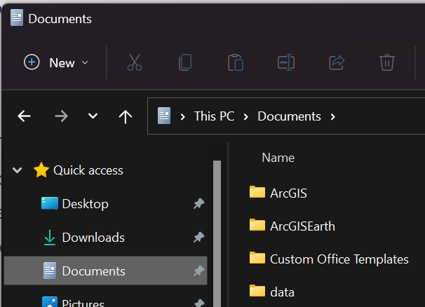
Note that in windows File Explorer, the Quick Access shortcuts go to the UNC path:
Documents folder accessed via UNC:
Documents folder accessed via Drive Letter (e.g., K:):
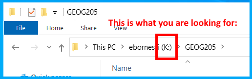
When opening your ArcGIS Projects ensure that (K:) is present in the file explorer breadcrumbs to ensure that tools will work as expected.
Opening ArcGIS Pro
This lab (and most labs throughout this course) will be completed primarily using ArcGIS Pro. The first time you open ArcGIS Pro (and potentially from time to time depending on automatic filesystem maintenance), it will need to be configured for licensing.
To do this:
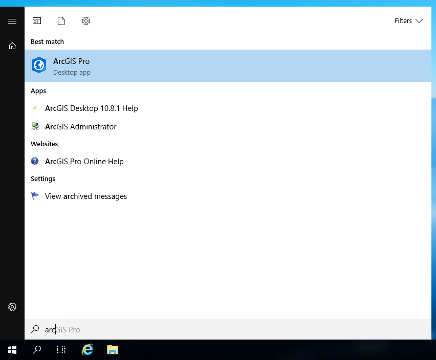
- Search for and open ArcGIS Pro in the taskbar
- It may open with a Licensing pop-up window
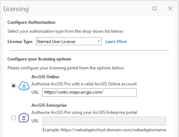
- Look at the bottom of the popped up window, click ‘Configure your licensing options’
- In the Licensing window, set up ArcGIS Pro licensing as the following (‘Named User License’ and https://unbc.maps.arcgis.com/):
You may be asked to close ArcGIS Pro and restart it to implement the changes.
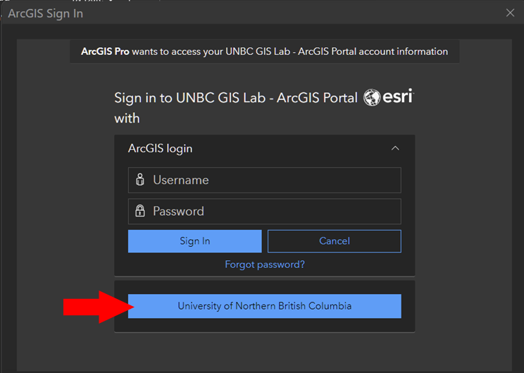
- On restarting the software, you may see a UNBC login window (select the blue ‘University of Northern British Columbia’ bar whenever you see it). Login with your UNBC email and password
- Once you login, you will see the ArcGIS Pro homepage. You will hopefully see your login name at upper right corner.
If not:
Log in to the ArcGIS Portal
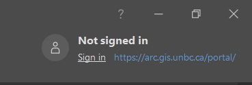
Throughout this course, we may be accessing data stored in our ArcGIS Portal. You will need to log into the portal to gain access to the data stored here. Once ArcGIS Pro is open, use the sign in button in the upper right corner to log into the portal at https://arc.gis.unbc.ca/portal.
On the login screen, choose the blue ‘University of Northern British Columbia’ button. This will allow you to login with your regular UNBC credentials. The default ArcGIS login is for legacy accounts and will not accept your UNBC credentials.
ArcGIS Pro Basics
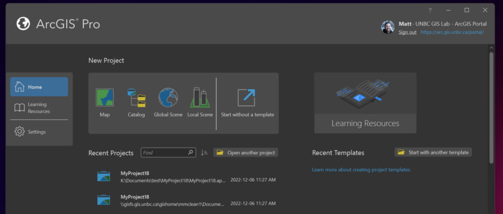
When you first open ArcGIS Pro, the welcome screen will present you with a variety of options.
In each lab, we will create a new project file to work in. Primarily, you will create projects by clicking on the map icon that creates a new project with an empty map inside.
A note about folder and file names:
GIS software can be very finicky in many ways (as we saw with the K: drive storage versus UNC file paths), and folder and file names are another example of this. Again, you don’t need to know why, but to prevent errors or unexpected results in your work, you should always exclude any spaces from your folder or file names. For example:
DO NOT: K:\Documents\GEOG 205\Lab 1\First Lab.atbx
INSTEAD: K:\Documents\GEOG205\Lab1\FirstLab.atbx
OR
K:\Documents\GEOG_205\Lab_1\First_Lab.atbx
Use underscores or capital letters to distinguish words in your folder or file names rather than spaces. As with the file storage location, making these mistakes will not produce error messages – that is, the software will not tell you not to do any of these things. Instead, you will run into mysterious errors later in the semester.
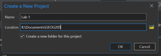
To make your first map, (1) select the map template, (2) give it a name, and (3) select where to save the project (K: drive). Inside your K drive, make a folder for GEOG205 – we will be saving all our labs here. Finally, (4) make sure to tick the ‘Create a new folder for this project’ box.
Once You Have Opened a New ArcGIS Pro Project
ArcGIS Pro overview:
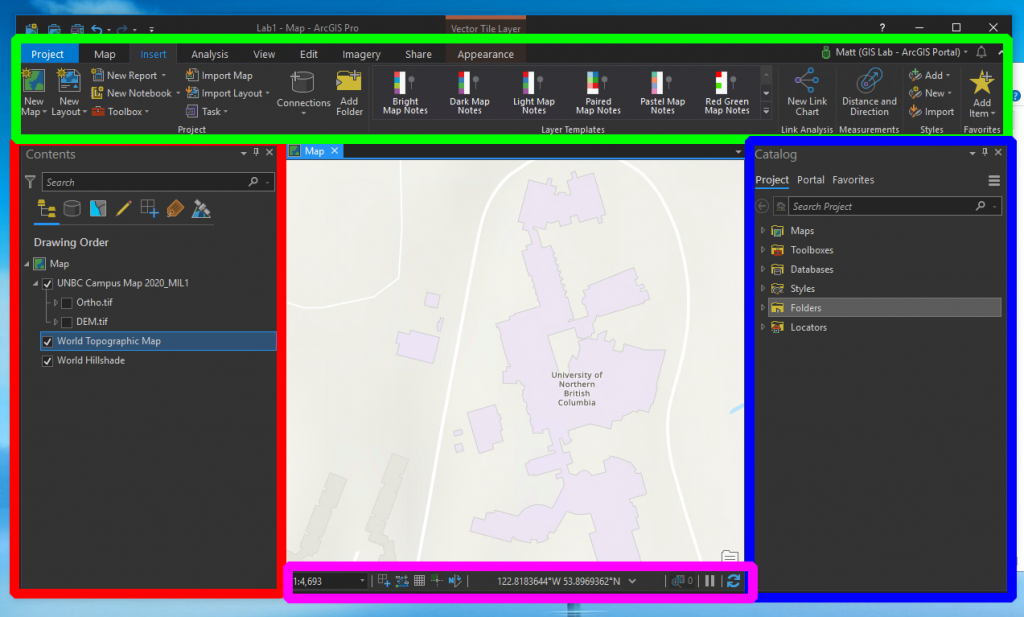
The ArcGIS Pro screen is divided into 5 primary sections:
1. The Map Viewer (the center space of the window – no corresponding coloured box in the ArcGIS Pro overview image)
In the middle of the window, you will see the map view. This is where all the data we are working with will appear, and you can navigate it much the same as Google maps, using click-and-drag and the scroll wheel on your mouse.
2. The Contents Pane (red box in the ArcGIS Pro overview image)
Moving to the Contents pane on the left side of the page, have a look at where it says Contents, then Drawing Order, then Map. Everything listed below ‘Map’ here is a separate layer in your project. You will notice that every map starts with a default ‘World Topographic Map’ layer and ‘World Hillshade’ layer. In the Contents pane, you can re-order your layers, you can organize them into groups, you can edit information about a single layer by right-clicking on it, and you can turn layers on and off using the checkbox next to each layer. For assignment submissions, you will often want to turn these two default layers OFF by unchecking the tick boxes next to each of them.
We’ll talk a bit more about the Drawing Order once we bring a few more layers into our project.
3. The Catalog Pane (blue box in the ArcGIS Pro overview image)
The column to the right of the map is the Catalog Pane. This is also where various tools will appear as they are opened. There are 3 tabs for accessing data here: Project, Portal, and Favorites. The Folders section in the Project tab gives access to data that is stored in the folder you created when making the project (at first, it will only have the project file that you just created).
To add data to your project, we need to first tell ArcGIS Pro where to find it. Right-click on Folders, then Add Folder Connection (you’re going to have to do this every time you start a new project). From here you will be able to select folders in the L: drive that you want to make available in your project. The two folders we will be using in this course are L:\DATA and L:\GEOG205. Add those two folders now, either one at a time, or by holding the Ctrl key to multi-select the folders, then navigate through the folders in the Catalog pane until you find the following file:
L:\DATA\PG_LiDar\pg_city_2010_lidar\UniversityAOI\Images\University_AOI_BE_15cm.tif
Add the file by dragging and dropping it onto the map.
Next, add:
L:\GEOG205\lab01\UNBC_Ortho_2021.tif
AND
L:\GEOG205\lab01\PG_Roads.shp
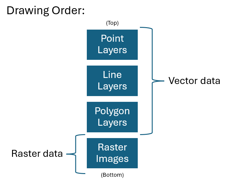
Currently, the UNBC ‘ortho’ image should be covering the greyscale LiDAR data, and the roads should be on top of all of it. If you want the LiDAR to be on top of the orthoimage, simply grab it and drag it above the UNBC campus map in the table of contents. This is what we mean by Drawing Order: layers that appear at the top of the list will be drawn on top of the other layers in the map viewer, and proceed in order from top to bottom. In general, it is best practice to keep raster layers at the bottom of the drawing order, followed by polygon layers, then line layers, with point layers on top.
Best practices for organizing data types in the ArcGIS Pro contents pane:
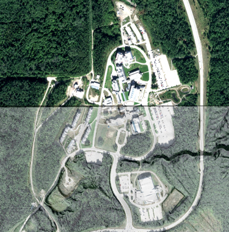
To illustrate the drawing order, we’ve made the LiDAR dataset (the greyscale one) cover only half of the UNBC campus. Let’s take it a step further and adjust the transparency of the LiDAR layer.
4. The Ribbon (green box in the ArcGIS Pro overview image)
To do this, we need to use the top ‘Ribbon’. Here the menus are sorted into categories of tasks, such as Analysis, Editing, and Sharing. When you have a layer selected in the Contents pane (the layer name remains highlighted blue even when you navigate your mouse away), there will also be additional menus added to the ribbon that are specific to that data type. For example, with the University AOI layer selected, as this is a .tif file, which is a type of raster, the Raster Layer tools will be available on the Menu.
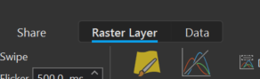
Open the Raster Layer Tab and set the Transparency (in the ‘Effects’ group of tools) to 50%, and you should be able to see the University campus behind the LiDAR layer.
5. The Info Bar (pink box in the ArcGIS Pro overview image)
Below the map is the info bar. In it, we see the map scale on the left, and towards the middle are the coordinates of the mouse pointer. Also take note of the ‘refresh’ arrows at the right-hand side of the info bar. This will display as a loading wheel when the software is working (for example, when loading a dataset or performing an analysis task). If it seems like something is not working or not loading in the software, check for the loading wheel first – it may just be thinking!
Scale Ratio Display:
There are many ways to change the scale or zoom-level of maps in ArcGIS Pro. Like we discussed above, you can zoom in and out using the scroll wheel on your mouse (holding the Ctrl key while you do this will give you finer control of how much you zoom at a time) and can pan around on the map by clicking and dragging.
If you want to set a specific scale ratio, click on the drop-down arrow next to the scale ratio in the info bar. Alternatively, you can click on the numbers of the scale ratio and type in the specific ratio you want to use.
Map Display Units:
The coordinate system used to display your mouse pointer coordinates at the centre-bottom of the screen will usually default to whatever coordinate system the first layer in your project was projected to. You can, however, change the displayed coordinate system to others like UTM, Decimal Degrees, or Degrees-Minutes-Seconds by clicking the drop-down arrow next to the displayed coordinates. Switch the map display units to UTM, then move your mouse northward along university way to see the Northings increase on the display. Move your mouse eastward to see the Eastings increase.
Question 1:
In metres (using UTM coordinates), estimate how far north UNBC is of the equator, and how far east UNBC is from the UTM zone centre (500,000 E) near Miworth. Once you have these distances in metres, convert to a more appropriate unit, like kilometres. Save your answer in a text document in your GEOG205 folder for safekeeping, and copy/paste your answer into the Comment box of your Moodle submission (no need to upload the text document this time, but you will upload a PDF map).
Preparing a Map for Print
Before we can print a map, we need to make a layout. Projects can contain multiple layouts. For example, if you will be printing the same map on different sizes of paper, you can create one layout that is formatted to look nice (that is, has appropriately sized lettering, etc.) on an 8.5”x11” page, and another, separate layout that will look nice on a poster-sized page.
To make a layout, open the Insert menu on the ribbon, select New Layout, scroll to the ‘ANSI – Portrait’ section, and pick Letter (standard paper size). At this stage, you should have a blank canvas to work with. Also on the insert tab, there is a tool called Map Frame. Select this and draw a box on the canvas where you would like the map to appear. Next, in the Contents pane, deselect all the layers except for the orthoimage of the UNBC campus. You should have something that looks like this:
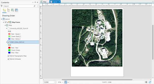
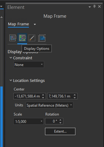
With the map frame selected (note the small boxes at each corner of the map frame that indicate it is selected), change the display options by right-clicking on the Map Frame entry in the Drawing Order, then select Properties. The Element Properties tab opens overtop of the Catalog Pane on the right-hand side of the page. Navigate through the icon tabs until you find ‘Display Options’ then set the scale to a round number that provides a decent view of the university campus. In this case, 1:5,000 works nicely.
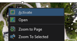
You can also adjust the extent of the image displayed within the Map Frame manually by right clicking on the frame (the image of your map) and selecting ‘Activate’. Notice now that the small boxes in the corner of the map frame have disappeared, and instead, all area that is not your map is greyed out.
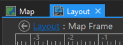
With your map frame activated like this, you can now click and drag, as well as zoom in and out on the map inside the frame. When you have the UNBC campus centered as you would like it, click the small red ‘X’ button in the top right-hand corner of the window to exit back to layout view.
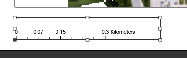
At this point, we have a general diagram of the University, but we want a map so we will add a scale bar, found in the Map Surrounds section of the Insert tab on the ribbon. Select a scale bar from the menu, then click and drag on an empty space on your page to generate a scale bar that is approximately the size that you want it to be. Once you create it, try making your scale bar bigger or smaller by clicking and dragging one of the corner boxes. See how it automatically recalculates the divisions in response to the changes you make.
When you add your scale bar, it will most likely show up with some messy looking divisions. For most people, 0.07 Km is not a meaningful unit of distance, and values less than/to the left of zero are not desirable. Let’s fix that.
With your new scale bar selected, use the Element panel on the right side of the window to change the units to something more suitable – in this case Meters* (Metres) would be a good choice. Note that this US software by default spells ‘Meters’ instead of Canadian spelling ‘Metres’ – bonus if you edit the Label Text to our proper language!
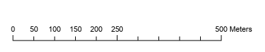
Change the width of the scale bar to make it 500m long. This is starting to be more useful, but at this point, we still have divisions every 62.5m, which is not great.
Navigate to Properties in the Scale Bar Element tab:
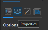
Change the number of Divisions and Subdivisions so that the divisions represent nice round numbers. In this case, I went with 2 divisions with 5 subdivisions, but you may find other combinations that work well. Additionally, you can change how the labels appear under the numbers section, using the Frequency Setting. As an example, setting the number frequency to ‘Divisions and the first subdivision’ produces the following result:
If you have more layers, it would also be appropriate to add a Legend in the same manner as the scale bar, but that will follow in Lab 4. You can add a North arrow in the top left corner of the map.
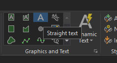
Finally, we will use the straight text tool to add a title as well as your name and the date the map was last updated.
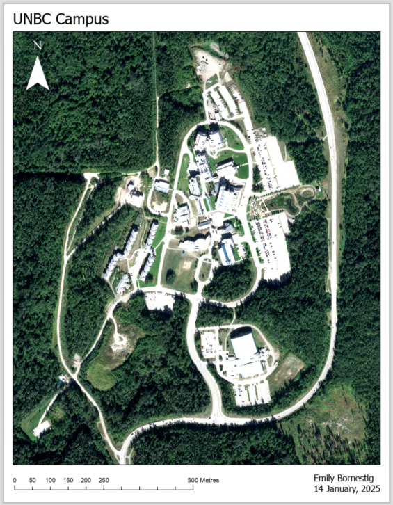
By the end of this class, we will be making much better-looking maps, but this serves as an introduction to the software we will be using.
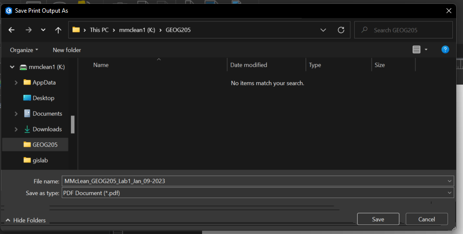
The last thing for today is to submit your map in Moodle. In the top Ribbon, go to Share, Print Layout, then set the Printer Name to ‘Microsoft Print to PDF’.
Save the PDF as <yourusername>_GEOG205_Lab1
Next, let’s proofread our work and make sure that the PDF exported correctly by opening the exported file in a PDF viewer (not in ArcGIS Pro). If it looks the way you expect it to (that is, the same as your Map Layout), go ahead and upload your PDF map into Assignment 1 on Moodle. Don’t forget to copy and paste your answers to Question 1 into the comment box of your submission.
Each week’s assignment is due before the start of next week’s lab.
Note: this map will not be graded, the submission is only to ensure the system is working, and you are able to access it correctly.
Expectations (Tips for Success)
- Arrive for your lab on time. We try to keep everyone on pace during lab, and it is not fair to make the class wait for you to catch up if you arrive late.
- If you must miss your lab section, please e-mail your TA ahead of time to let them know not to expect you. Provided there is room, you are welcome to sit in on another GEOG205 lab section for that week. Check the UNBC GIS homepage for the lab schedule.
- Stay for the whole lab, or until your assignment is done. Your lab time is a great time to work on your assignment as it is already scheduled, and it is easy to get help from your TA during lab section.
- Assignments are due before the start of your next lab. This is for your benefit, as the labs are designed to build on one another, meaning that the skills you practice in Lab 1 will be needed to complete Lab 2, and so on.
- Once your lab starts, last week’s assignment is already late. You are encouraged to be present for the current weeks content, then finish the previous assignment later that day if you need to.
- Assignments have a 20% (1 mark out of 5) penalty per day late. (If you are unable to complete an assignment on time for a justifiable reason, e-mail your TA and Dr. Wheate before the due date; it is much easier to offer extensions before your assignment is late).
- When working on your assignments, read the instructions thoroughly. In this course, formatting details matter. In the workforce when producing maps, they will be expected to be not only correct, but in the correct dimensions and file format requested for publishing. Before submitting assignments, you should always proofread them in the final submission format (e.g., open the PDF file you created in a PDF reader like Foxit or Adobe, or in a web browser):
- Use the assignment instructions as a checklist: are all required components present as described?
- Does the map reflect cartographic principles you have learned in lecture?
Pay special attention to the concept of today’s lab. - Should you have a north arrow (maybe not, more on this later), and is your scale bar in logical units?
- Do your layers show up in the legend with display labels (as opposed to underscores and abbreviations – see later labs)
- Maps are a communication tool, what does your map communicate?
- Is your map visually appealing? Cartography is an art form.
- Open your PDF in something other than ArcGIS to ensure it rendered correctly.
- If you have questions, please ask. You are likely not the only person with that question. We aim to create an environment where you feel comfortable asking questions and engaging with the lab content.
- Also note that instead of office hours for this course, your TAs will be available for support by appointment. Reach out to them in lab or by email (Emily: Emily.bornestig@unbc.ca; Dinesh: dbhatt@unbc.ca). Ping will also be hosting open drop-in times in the GIS lab on Tuesdays from 9:30 – 11:30, Wednesdays from 9:30 – 11:30, and Wednesdays from 14:30 – 16:30.
- NEW FOR 2025: The GIS lab will no longer be available to students after hours. Instead, your work and the GIS software can be accessed from any computer on campus or on your personal computer by accessing Osmotar (details here).
- If you find that the existing drop-in times are not working for you and you need more open lab time during the week to work on assignments, please reach out to Dr. Wheate and your TA, and we will set something up.