Working with ArcPro
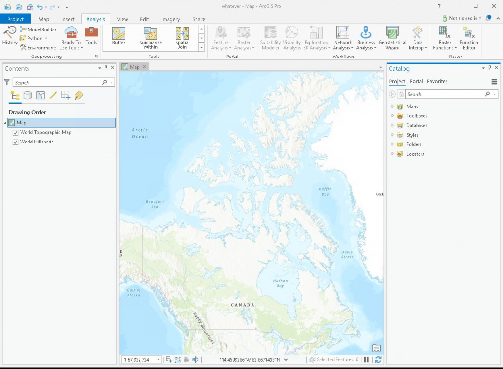
This week’s lab is going to use ArcPro, a world leading GIS software used by industry, government and many commercial companies. ArcPro and QGIS are very similar in how they work and the layout of the software.
Starting the software is the same as others, under the ArcGIS menu launch ArcGIS Pro. If a SignIn window popup or license requirement, please check the website to set the license for ArcGIS Pro https://gis.unbc.ca/support/licence-arcgis-pro/ (Note, you will need to restart ArcGIS Pro after license configured)
Once you start ArcGIS Pro, Set up a workspace for this week’s lab:
- Click Map under the New column
- Create a new project and folder in your K:/geog204 folder called lab3 (very inventive)
Setting up folders for use in your project
Once ArcPro is open you should have a menu on top, a map in the middle, the table of contents (layers panel) on the left and the catalogue (browser) on the right.
Set up folder connections in the Catalogue panel by:
- Right click on Folders
- Add Folder Connection
- Navigate to L:\GEOG204 folder and click OK to add the GEGG204 folder to the list for easy access
ArcPro Analysis
Simple Query based on Attributes
In this lab, you will be exploring more functionality available in ArcGIS and learn basic analysis skills.
Add the following datasets from L:\GEOG204\lab3 folder
fcover, trails, lakes, wetlands
Finding the area with ‘spruce’ as the leading species
- As with QGIS, right click on the fcover layer and open the attribute table
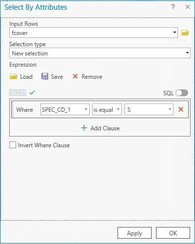
- Choose Select by Attribute in the top menu of the table panel
- Set up a new selection
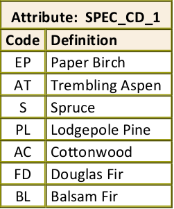
- Select for SPEC_CD_1 equal to “S”
This follows the naming conventions for forest species:
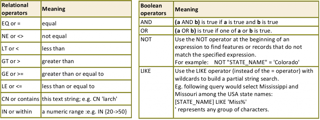
Using the an operator as defined below:
Finding the areas that have Spruce as the leading species, stand age greater than 30 years and the leading species cover 70% of the area
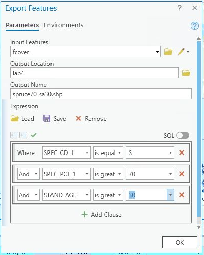
Use the query builder (use the Add Clause button) or type in the following expression in the query box
(“SPEC_CD_1” = ‘S’) AND (“SPEC_PCT_1” > 70) AND (“STAND_AGE” > 30)
You will save your new selection to a shape file on your K: drive by repeating the selection in the export tool by:
- Right-click on the fcover -> Data -> Export Feature
- Save your output feature as spruce70_sa30.shp in your lab3 folder
- ENSURE you add the .shp to the name of output (this will provide a shapefile as a result)
Finding the distance from points to the nearest line features
In some cases, we want to know the spatial relationship between features. For example, with our sampling plots data, we want to know if a water source has a big impact on the growth of trees. In other words, we want to know if the trees that are close to a water source grow better than those that are further away.
Add the creeks and sample data to your project from the lab3 folder in the L:\GEOG204 folder (you may have to refresh the folder in catalogue).
Perform the selection by:
- Access the Analysis tab on the top of ArcPro
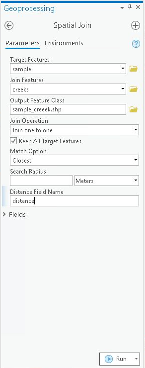
- Select Spatial Join and set it up using the information and image below:
- Use the sample layer as the target feature
- Use creeks as the join feature
- Rename and check the save location of your output in the Output Feature Class section
- Make sure the Join Operation is ‘Join one to one’ and the Keep All Target Features box is ticked
- Match option is Closest (not Closest geodesic)
- Set a field name for the distance (i.e. “distance”)
- Click Run
The resultant attribute table will have all the attributes of the nearest creek, and the distance as the first of the new fields.
Try another query using the table selection (right click on the distance field, then Sort Ascending) or Select by Attributes again to see how may sample points are within 5 meters of a creek.
Note: You will probably still have an attribute table open at the bottom of your ArcGIS window from before, but look at the tab at the top of the attribute table – which layer does that attribute table belong to?
Line-on-polygon and polygon-on-line selection
Sometimes we need to know which line feature overlays the polygons with specific attributes. For example, which creeks (water sources) pass through young to middle aged forest stands (polygons). Use the layer you created when you queried the spruce trees and select the creeks that pass through these polygons.
- Click Map from the top menu -> Select By Location tab.
Input Features: creeks
Relationship: Intersect
Selecting Features: spruce70_sa30
Leave everything else as they are and click OK
Test your skills by combining a selection
Now try a new selection using the Select Layer by Location tool with the following criteria:
- Load the bird_nest layer from the L:GEOG204\lab3 folder
- Use the orginal fcover layers (not your species and age forest cover layer)
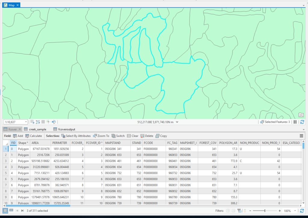
- Find which forest cover polygons intersect with the bird_nests layer
- From this bird presence fcover selection, select (subset from the current selection) which polygons have lakes in them
We are looking for fcover polygons that intersect with both bird_nests and lakes (this should give you 3 selected polygons):
Overlay Analysis
Spatial overlay is a process whereby themes or datasets sharing the same spatial extent are compared with resultant layers produced. We are essentially comparing the simple feature locations of different layers.
In GIS, where lines intersect between one theme and another, vertices are created. Where lines or points share the same space as polygons, the lines and points inherit the attributes of the spatially corresponding polygons. New layers are formed which can take on the attributes or coordinate properties of input datasets. Some or all features and attribute values from the input datasets are passed on to the output. Overlay analysis is multi-layered analysis and the operations modify the geometry and generate a new dataset.
All the datasets required for this part of the lab are located at L:\GEOG204\lab3
| Dataset | Description |
| bird_nests | Bird nest locations around Forests for the World |
| creeks | Creeks |
| wetlands | Wetlands |
| lakes | Lakes |
| fcover | Forest cover data |
| trails | Trail system |
| slopes | Slope and aspect data of the terrain |
| bndy | UNBC map boundary |
We will be starting a new map in ArcPro and saving it as Analysis
- Click Insert-> New Map. A new map called Map1 will show in the display area just like the first default Map.
- Right-click Map1 in the table of content-> Properties. Rename the Map1 to Analysis
- Add all the layers mentioned above to Analysis map
- Turn off the visibility of the slopes layer
- Adjust the order of your loaded layers so you can see your points and lines on top of the polygons
- Resave your map – you can just hit the save button on the very top of ArcPro (ctrl + s)
Buffering
The Buffer tool creates a new output by generating buffer zones around input features. Input features can be polygons, lines, or points. Output features will always be polygons.
Assume that young birds often search for food within 50 meters of their nest while the older birds search for food within 100 or 150 meters of their nest. We can use the buffer function to determine the area where we expect birds to occur frequently. We will create two buffer datasets on bird_nests.
Buffer bird_nests at 50 metres
- Activate the Analysis tab on the main menu
- Search out Buffer in the geoprocessing tools
- Set up your analysis accordingly:
Input Features: bird_nest
Output Feature Class: birds_buffer50.shp
Distance: 50
Linear Unit: Meters
Method: Planar
Dissolve: No Dissolve
You should now see some round polygons around your birds nests. You can zoom in by switching back to the Map tab and using the navigation tools.
Buffering with multiple buffers – 50, 100, 150
- Find the Multiple Ring Buffer tool
- Add in the values accordingly:
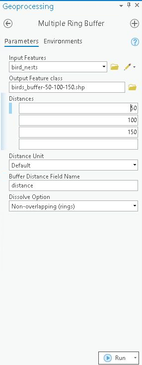
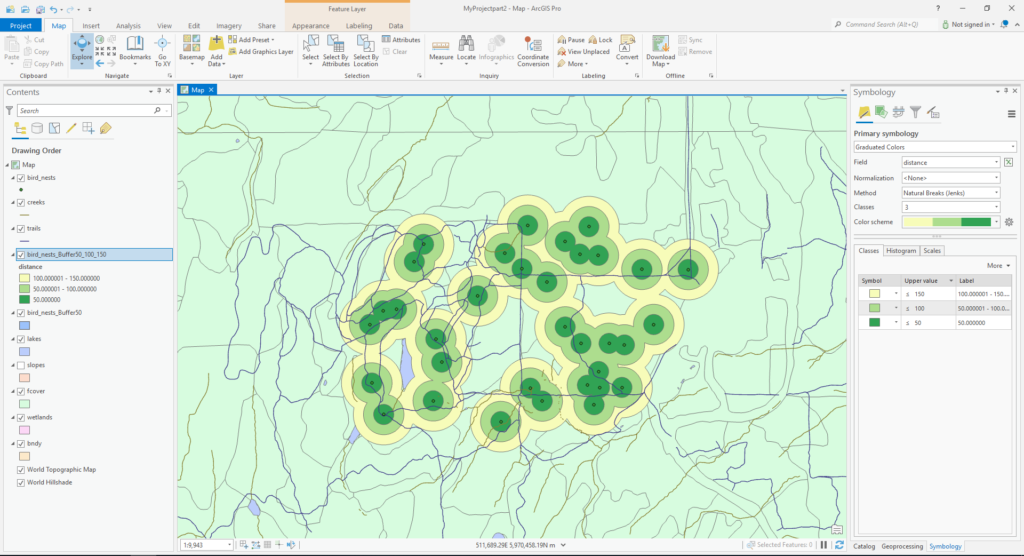
Examine the attribute table of each buffer dataset (ie. birds_buffer_50 and birds_buffer_50_100_150). The data field Distance is generated automatically for the multiple ring buffer dataset.
Style your new layers. Right click the layer –> Symbology. Select Graduated Colours, then explore the fields, classes and colour schemes until you find something you like. Double click on the cells for ‘Upper Value’ to set a more appropriate number to classify by (leave the final cell the same as it automatically populates to the largest value detected).
Intersecting
We are going to perform an operation to extract where the geometries of two layers intersect with each other. Check out ESRI’s description of intersect.
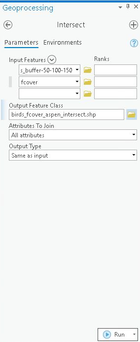
We want to know the area with Trembling Aspen (AT) as the primary species that falls into the 50 meter buffer of bird nests. To solve this problem we need to use the Intersect tool.
The Intersect tool overlays two datasets to create a single output. Only those features that occupy the same spatial location in both datasets will be preserved in the output dataset. The features in the output dataset will have all the attribute data from both input datasets.
Select by Attribute
For the question mentioned above, you need to first perform a Selection by Attributes on fcover to get the area that has ‘Trembling Aspen’ (AT) as the leading species. You did this for “spruce” before, just substitute ‘AT’ into the expression:
“SPEC_CD_1” = ‘AT’
Intersecting:
- Select trembling aspen in the fcover layer
- Find the intersect tool in the geoprocessing tools
- Add both the layers in as inputs
- Run
If all went well, you should have the intersections of the selected fcover layer with the buffered birds.
Check the attribute Shape_Area which provides the updated area value
Explore the basic statistics of different fields in your attribute table by right clicking on the field header –> Statistics. The right-hand side of the page will list the basic statistics, including the sum (take note), of the field you chose. If you have some but not all records (rows) of the attribute table selected, the statistics will reflect your selection only.
Clipping
Clipping is a frequently used spatial overlay tool. It is similar to intersecting, but it is used to extract the features and attributes of one layer, using a second layer as a “cutter”. The result is a subset of the input layer, compared to intersecting which combines two layers in shared geometries. Check out the GIS wiki explanation of clipping.
In some cases, a dataset covers a much larger area than we are interested in. In this case we can use the Clip tool to clip the trails line layer with the bndy polygon layer. The bndy polygon is the “cookie cutter” in this case.
Clipping trails with the study area
Clipping follows the same procedures as the above overlays:
- Find the CLIP tool in geoprocessing
- The input feature is trails
- The clip feature is the bndy layer
- Output Feature class: trails_clipped_bndy.shp
Assignment #3 – 5% due next week
In this assignment, you will perform GIS analysis for the Forests for the World area. You will:
- Identify the level of difficulty of trails based on slope degree
- Identify potential campsite locations in relatively flat locations along the trails and lakes
HINT: Hover your mouse over the ‘info’ icon next to the different input sections of the tool you are using to help you choose which boxes to put which files in.
The data needed for this assignment are:
ffw_bndy, lakes, trails, slopes
ffw_bndy is the park boundary the Forests for the World. As we are only interested in the Forests for the World area,
- clip lakes, trails, slopes using ffw_bndy as the cookie cutter, saving them as lakes_ffw, trails_ffw, slopes_ffw respectively
Use your clipped features for all further analysis:
1. Use slope degree to categorize trails into ‘easy’, ‘medium’, and ‘hard’:
- Intersect the trails layer with the slopes layer to assign slope values to each segment of trail
- Recalculate LENGTH (use kilometers as the unit)
- Change the symbology of the resulting layer based on the slope value (Degree_SLO) in graduated colour with 3 classes:
- Easy: less than or equal to 5
- Medium: less than or equal to 15 but greater than 5
- Hard: greater than 15
- Question 1 (1.5 marks): Record the total length (sum) of each trail class. Include the units you used! (0.5 marks per trail class)
2. Locate the potential campsites along the trails and lakes (1 mark)
The potential campsites need to meet the following criteria:
- Must be within 20 meters distance of trails and Shane Lake (the biggest lake in our clipped layer)
- Should be in a relatively flat area (slope less than or equal to 5)
Step 1: Locate the 20 meter area along the trails using the buffer tool. Make sure to dissolve the output into a single feature.
Step 2: Create a 20 meter buffer around Shane lake. Set Side Type to Exclude the input polygon, this will exclude the waterbody area. In the attribute table of your buffer output.
Step 3: Filter out the area with slope less than or equal to 5 degrees in your slopes layer.
Intersect the results from steps 1, 2, and 3.
Question 2: Note down the total (sum) area for the potential campsites. (1 mark)
3. Produce a map (export as image, or take a screenshot) to include in your write-up: (2.5 marks)
- Check the boxes in the table of contents pane to display the map layers you want to include in your map
- Insert > New Layout > Choose an appropriate page size (ask Google if you need guidance)
- Map Frame > Default Extent > Click and drag a map
- Your map should include:
- 0.5 marks: Trails coloured by difficulty level
- 0.5 marks: Your potential campsite polygons and your not-buffered lakes layer
- 0.5 marks: An appropriate legend
- 0.5 marks: Map title, scale bar, north arrow, and your name
- 0.5 marks: Overall layout
Save your answers together with your map as lastname_firstname_geog204_A3 in a MS Word file and submit it to your TA through Moodle