Raster data as spatial layers
In this lab we are going to look at some types of raster data as well as exploring these data in both QGIS and ArcPro.
Starting with QGIS
Load the crop inventory file
Open a new project and add the raster file (aci_2019_bc.tif) from L:\geog204\ lab4/cropinventory folder. You can do so by dragging and dropping or by:
- Layer -> Add Raster layer
- Navigate to the L:/GEOG204/cropinventory folder and load the aci_2019_bc.tif file
Let’s look at how this raster layer differs from vector data. See how a raster layer is made up of cells or pixels, and it displays the range of cell values in the Layers pane.
Note also that there is no attribute table affiliated with the raster layer. Instead, each cell has a value, which represents the data we’re going to make use of in today’s lab.
Click the Information icon, then click anywhere on your raster layer. See the window on the right of the screen – it will tell you the value of the cell you clicked on. What is the value of the black space around BC? What is the cell value of water?
Try styling the layer to visualize it better:
Style the layer
- Right click ->Properties -> Symbology -> Palleted/unique values
- Select a colour ramp, Browns to Blue Green works well enough (BrBG)
- Classify – hit the classify button
- Remove the first two values (0 and 20) using the red ‘minus’ button
- Hit OK
What is the most common value
Once the data is loaded and styled you can visually see the crop classifications in British Columbia. Check out the histogram (counting out the number of pixels of each type of crop)
- Go to Layer Properties -> Histogram tab on the left panel, then ‘Compute Histogram’
There are two values that have a large spike in the count of pixels, one is 0 (non-values), what is the other value? If you hover over the bottom axis, you can see a magnifying glass allowing you to click and drag to zoom in along the axis. You can right click to zoom back out.
Add some data to determine crop type
there is a table that references the type of crop to the pixel values. We can also load a table in the same folder as the .tif file into our project that has this reference.
- Load the aci_2019_bc.tif.vat.dbf file into your project and check out the (attribute) table.
Question 1: (1 mark)
What pixel (cell value) has the greatest count (0.25 mark)? What is the type of crop with the greatest count (0.25 mark)? what number type is this raster data (0.5 mark)?
Question 2: (1 mark)
What is the pixel size of the dataset in meters (0.5 mark)? How could you figure out the area covered by the different crop types by knowing the number of pixels of each value (count column in the table) (0.5 mark)?
ArcPro
Open the same dataset in ARCPro.
How are the data styled in ARCPro? It makes use of the crop inventory table (aci_2019_bc.tif.vat.dbf) to create the styling.
- Load in a DEM (Digital Elevation Model unbc_dem_alb.tif) located around UNBC.
- In the unbc_dem folder folder for this lab, add the unbc_dem_alb.tif file to your ArcPro project. Zoom to this layer and play around with the styling.
Creating some terrain layers
Create a slope layer
Switch to the analysis tab in the ribbon and type ‘slope’ in the search field in the geoprocessing panel. Create a slope layer called unbc_slope.tif (or unbc_slope_arcpro.tif)
Input raster: unbc_dem_alb.tif
Output raster: unbc_slope_arcpro.tif
Output measurement: Degree
Using the Raster Calculator
Search the geoprocessing panel for “raster calculator” and launch the tool.
Using the raster calculator on a raster layer is similar to selecting by attributes on a vector layer: we create a query that gives conditions for what we want to extract from the original layer. Building queries works the same way here as it does with querying vector layers, only the output is saved to a new layer rather than selected.
Note that you can use the raster calculator to build a query that draws on multiple raster layers at once, and creates a single output based on selections from all referenced layers. For now, though, we’re going to just use one.
unbc_slope_arcpro.tif <= 10
- Save the output raster as unbc_slope_lt_10.tif
How do the results look? Consider the query that you built, then consider the output. It only produced two values (a binary output): those that did not meet the criteria that you set out in your query, and those that do. This layer has pixels (from the slope layer) that represent areas that have either slopes greater than 10 degrees, or slopes that are less than or equal to 10 degrees.
Question 3: (1 mark)
What is the number type of the DEM layer (0.25 mark)? What is the number type of the layer from unbc_slope_arcpro.tif layer (0.25 mark)? Which value in this layer represents slopes less than or equal to 10 (HINT: Look at the layer and compare it in your mind to what you know of Prince George – which parts are hilly and which are flat?) (0.5 mark)?
QGIS
More Terrain Layers – QGIS
Back in QGIS, load the unbc_dem_alb.tif layers into your project.
Aspect
Create an aspect layer using the “aspect” tool in the processing toolbox.
Elevation layer: unbc_dem_alb.tif
Aspect: unbc_aspect.tif
You have now created a layer that represents the direction the cell is facing (the slope of the cell) in regards to north-south-east-west.
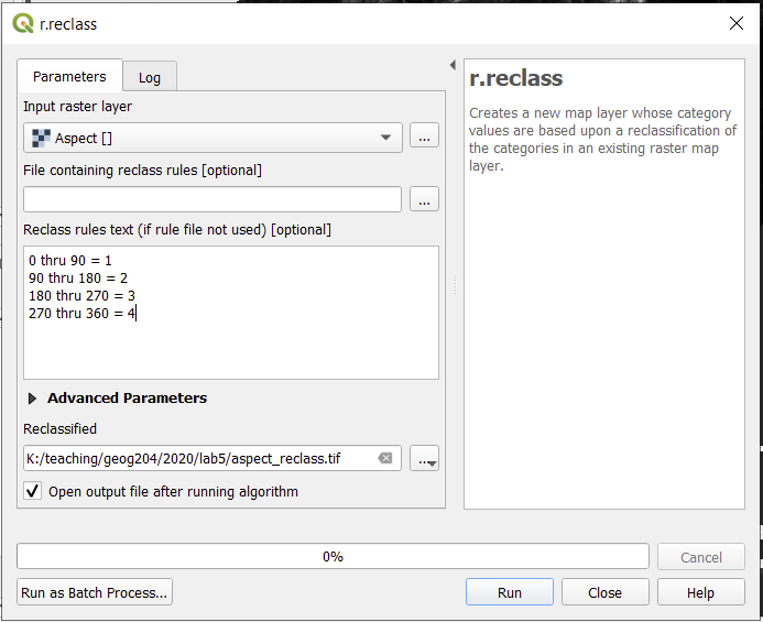
Reclassify your data
We’re going to reclassify the data using the r.reclass tool in QGIS (which is a GRASS function). Change this aspect layer into 4 classes (four quadrants that represent NW, SW, SE, NE). This is only one method of classification – but it works pretty slick (use the image below for an example). Call this layer unbc_aspect_reclass.tif
Raster Calculator in QGIS
The raster calculator for QGIS can be found in the top Raster menu
Raster –>Raster Calculator. You can use it, or the one in ArcPro to carry out the question below:
Question 4 (2 marks):
This is a two mark question performing the follow raster data query.
Using the raster calculator, provide a resultant layer that meets the following requirements:
- A Coniferous crop classification in the crop inventory layer aci_2019_bc (0.5 marks for this part of your query)
- Slopes less than or equal to 10 degrees (0.5 marks for this part of your query)
- South facing (aspect: 135 – 225) (0.5 marks for this part of your query)
Take a screenshot of your result (0.5 marks) and provide the query you used in the raster calculator (see mark breakdown above).
Save your answers together with the screenshot as lastname_firstname_geog204_A4 and send it to your TA through Moodle