Topics:
- Devising a model to solve a geographical problem
- Access to spatial and attribute data through the UNBC Library
- Defining Stats Can boundary files and connecting data to them
- Building a query that exemplifies our model
Solving a Problem
We have been working toward gaining some understanding of the many aspects of spatial data, and how descriptive information can be linked to these geographical entities. Today we are going to take a break from GIS theory and concentrate on GIS applications. This is where we start to think about the mechanics of applying GIS tools towards your project ideas.This lab will not be as involved as your project, but it brings together what you have learned so far to aid you in forming an idea of how to approach your project.
We will work with Stats Canada data to test a simple theory of how well distributed hospital locations are in regards to preconceived medical notions. We are going to assume that we have done our background research (lit review) and we are going to build a model based on population descriptors expressed spatially. We are going to look at the distribution of people within parcels of B.C. We then will look at the distribution of hospitals in these areas.
- Make a folder lab5 for today’s lab
- Open a new QGIS project, go to L:/GEOG204/lab5 and load up the two datasets listed below
- – dabc
- – hospital
- Arrange the layers so that both layers are visible.
Check out the illustrated glossary to find a description of this census layer at Stats Can illustrated glossary > Dissemination Area > Dissemination Area (in the Dictionary, Census of Population, 2016). We reviewed these small area stats can boundaries in last weeks’ lecture, and we will review these more in our next lecture.
Question 1 (1 mark): What is DA an acronym for (0.25 marks)? What parts are combined to record a DA as a geographic code (0.25 marks)? Provide an example code for a DA in Prince George (0.5 marks). Dissemination area: Detailed definition
Aggregation of Stats Can data (a different geographical level of Stats Can data)
We will use attributes to get a better understanding of how smaller units can be aggregated to larger census units.
We can use several methods to aggregate individual DA units into larger community based conglomerates (such as Fraser Fort George Regional District), which can help us determine the population ratios that hospitals have to support.
Before we aggregate data, review the attribute table for the dabc layer. What are the items in this table? Do they have some meaning to you? Can you determine which fields in the dataset have unique identifiers and what they are? Can you determine if this identifier is a character (text) type or numeric type (by looking to see which side of the cell the values are aligned with)? If you chose the “DAUID” as the unique ID based on your knowledge of Stats Can geography naming – does it work as a UID in a GIS table (are all the values unique)?
Zoom into Prince George. Use the information button or the select feature tool – and click on a DA unit in the city.
Question 2). Three parts for 2 marks
Some of the DAUID values are not unique – why is that?
HINT: In the attribute table find two DAUID values that are the same, highlight them both (remember that you can hold the ctrl key to select multiple values), then zoom to the selected values (there is a zoom to selected button) (0.5 marks)
Why are there ‘NULL’ values for DAUID and other attributes?(0.5 marks)
Based on the DAUID value, determine the Census Division (CD) value for Prince George (0.5 marks). From this, explain how to aggregate all the DA units into a single Census Division (as a selection or shapefile) based on the DAUID (the concepts, not the QGIS commands) (0.5 marks).
HINT: Write up the steps you take below:
Using the query function to aggregate DA units to a CD unit
We need to use the query functions (‘Select Features Using an Expression’) in the attribute table for the “dabc” layer. There are some helpful hints for this such as:
- With numeric columns (aligned to the right), you can use operators such as > or < with the conjunction operator ‘AND’ to squeeze out the Fraser Fort George Polygons’. As an example if the PRCD was 1234 we could use the expression:
“DAUID” >= 12340000 AND “DAUID” < 12350000
- you can use the operator ‘LIKE’ to compare a field to character values the % acts a wild card (can be any character); as such you can enter the part that will be consistent, followed by the wildcard.
“DAUID” LIKE ‘PRCD%’
- another way to query is to use the column filter (in the pull down menu in the bottom left) for DAUID and just type in the value you are searching for. Once you have performed the query and selected the values from the table – you should have something that looks like this:
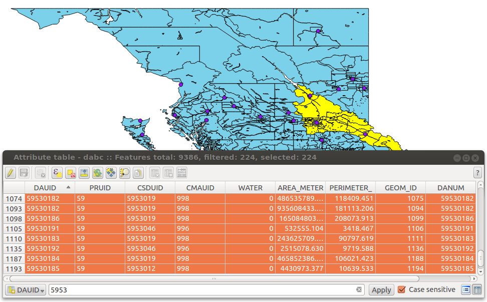
- Save this newly created subset (the Fraser Fort George CD, 5953) as a new shapefile in your directory.
New Boundary data and Attributes for your aggregation
For this lab we will use all of statistics for B.C. to match to the new Fraser Fort George CD. Can we do this? The table from Stats Can will have many more records (rows) than the attribute table for the CD layer.
Download a Boundary file from Stats Can
Open a web browser and search for ‘census boundary file 2016’.
- English data
- shapefile format (.shp)
- Dissemination Areas
- Cartographic file
Save the downloaded file (a compressed zip file) into your lab5 folder:
- Go to your lab5 folder
- right click to decompress the files into your lab 5 folder
- add the new data layer into QGIS
Zoom back into the area around PG. Notice the difference between the shapes of the polygons between the layer you loaded from the lab folder to the new file you have downloaded.
Subset the BC DA polygons
The census data gathered for the section below is for BC only, but the census data we just downloaded is for all of Canada. With this in mind, we should create a new shapefile from the downloaded dataset that has only the BC polygons.
- Select the BC data from census data layer and export it as bc_census2016DA
- Once you have extracted your BC subset, remove the census data layer
Joining census values to boundary files
To keep us all on the same page, we will use the data prepared for the lab (a non-spatial *.csv file for importing into QGIS like we did in the first lab).
Add da_pop_all_of_bc.csv from L:\GEOG204\lab5\census_data
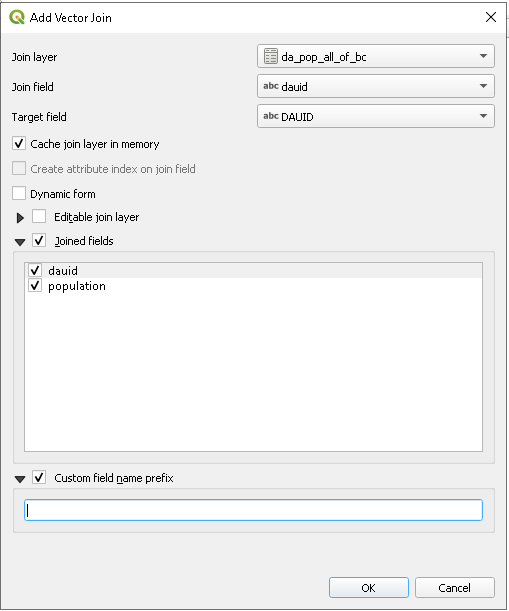
Join the two tables together (your new CD layer and the CSV file) in the following manner:
- Right click on bc_census2016DA and open its properties
- Go to the joins tab
- select the layer to join and the fields to join on (see screenshot below)
- Choose the fields that are joined to the table (“Joined fields” tab)
- Set the “Custom field name prefix” to be empty as the image shows below:
Calculate population density
Once you have joined the data together – open the data and observe that some of the population values are “0 or n/a”. What could create these values in a DA census set?
Clean your data to remove “n/a” value
Now that find any polygons that have an “n/a” value and delete them (don’t forget to Toggle Editing Mode). Once selected you can hit the red garbage can to delete the row, then save your edits.
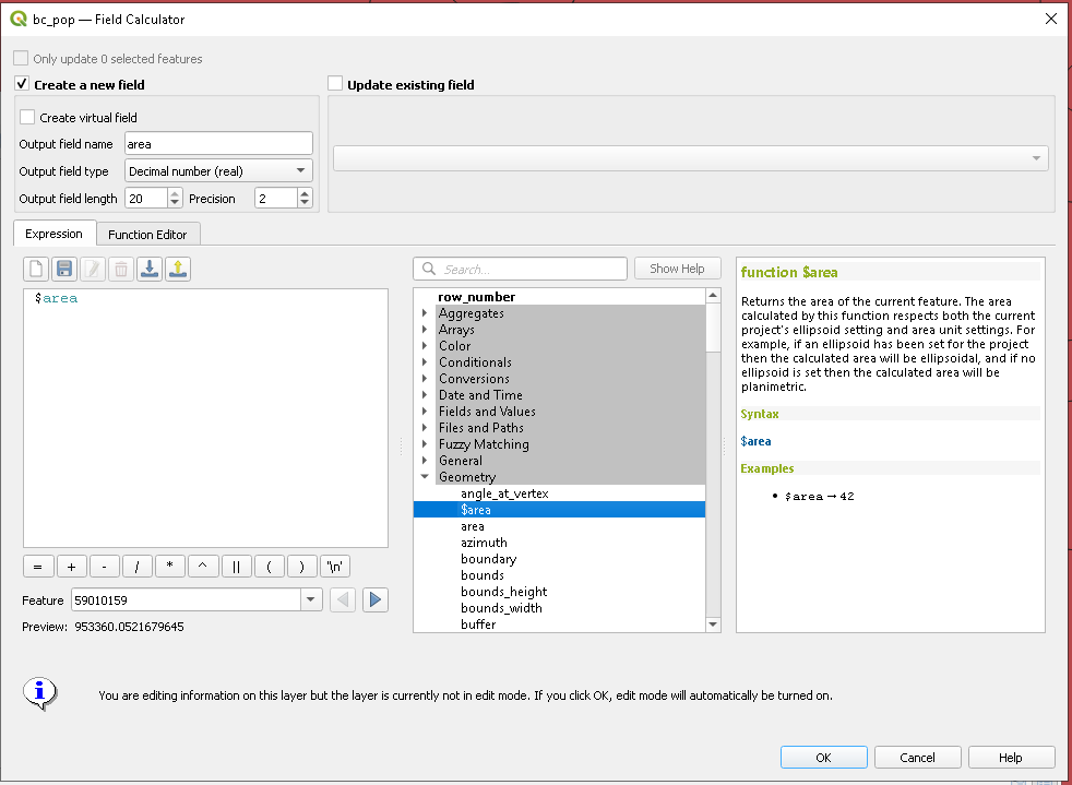
Calculating the area of your DA polygons
We also need an area for the polygons to calculate population density.
- Open the attribute table of your layer
- Find the field calculator button and launch the calculator
- Set up a new field called Area as a decimal number with an output length of “20” and precision of “2”
- Use the “$area” geometry function to populate this column
- Use the image below as your guide
Calculate population density
Now that you have population values and area, calculate the population density of the polygons in square kilometers by:
- opening up the field calculator and create a new field
- create the new field called popdense
- Decimal number with precision “2”
- use the calculation
- pop / (area /1000000)
Save your edits to the shapefile.
Make a simple map to show the population distribution
Style your Census Division values
As you did in the first lab, style your BC DA layers using the “categorized” option with your population field as the field to classify with. Here is a quick reminder as to how to do this:
- Right click –> properties
- Click the symbology tab and switch to categorized from single symbol
- Use the CDUID column
- Hit classify
- Apply and OK
This is really not a good looking map, but it will work for what we need to do today. A better map would be to use the graduated styling method using the population values. In order to do this, you would need to change the population values to integers instead of text values.
- Add a new field ‘POP’ with integer type (15 digits)
- Assign the value of population from the joined table to this POP field (“POP” = “da_pop_all_of_bc_population”)
- Symbolize the layer using POP field in Graduated color with 5 class and natural break method
Now let’s change the display coordinate system to make the map look better
- Click Project->Properties.CRS and choose BC Albers (EPSG 3005) as the display coordinate system.
Q3. Make a simple map showing the BC 2016DA population distribution with proper title, legend and scale (1 mark) Take a screenshot
Export your results to Google Earth
You can export data to Google Earth (KML file) at any time using the right click –> save as method – BUT this method does not save the styling for polygons. We are going to use another plugin to get the styling as well.
Plugins: Add the plugin mmqgis to your project
Here are the steps to export the map to Google Earth
- Add the mmqgis plugin as usual
- Click mmqgis menu –> Import/Export –> Google Maps KML Export
- Choose the POP as the Name Field
- Set your filename and save location to your K: drive
- Click APPLY
- Wait until the bar turns blue giving you the number of polygons
- Hit CLOSE
Now Open up Google Earth and load the KML file into it
- Open Google Earth –> Menu –> Internet –> Google Earth
- File –> Open –> browse to your KML file
Question 4: 1 Mark
Take a screenshot of your Google Earth creation and paste it into your word file for this week’s lab assignment.
Assignment #5 – 5% due next week
- Save the answers for the 4 questions for this lab in a Word document labelled as lastname_firstname_geog204_A5.
- Submit your answer through moodle to your TA by next week’s lab session.