Introduction
Today we will be looking at doing GIS inside of the Enterprise Database using PostGIS. Now you may be wondering what is our motivation to using PostgreSQL and primarly it is due to its performance and concurrent access.
When we talk about performance we are talking about how many IO operations we can perform per second, in many of the datasets you have used in your classes to date this was not a large limitation, however as datasets grow we start to get more and more objects stored within a layer. As an example as a shapefile begins approaching is maximum filesize of 2GB querying a feture will take multiple seconds even if no joinst are involved. In a postgres database this same query will likely be measured in fractions of a second.
The other big advangate is concurrent access, generally when working with files only one person may edit a file at a time, but what if you were doing a survey and wanted several serveyers adding their data at the same time. Or what if you wanted to be able to continually add data and have end usersers always get the most recent edits? A Database management system (DBMS) provides this access for many users to be accessing the same data at the same time, with different permission levels.
Import Data from Stats Canada
We have downloaded some data from Statistics Canada to be used in conjuction with layers from other tutorials and labs.
Using the link below, grab the files from the statscan_boundary_files folder with the file name starting with blocks. If you have not downloaded the fire polygons from last week – grab the zip file from the fire_polygons folder as well.
https://fileshare.gis.unbc.ca/index.php/s/NmT5iDW4awTezfp
Stats Can Block data
The blocks boundary file you downloaded is the smallest (highers spatial resolution) polygons from StatsCan. There are no meaningful attributes in the data set until you join the population from census data (the csv file). We will prep the data and load it into PostGIS.
Before we start with working with the block data
We will open up two instances of QGIS in order to double of work speed – well maybe…
Wildfire polygons
In one instance, load in the fire polygons and load them into PostGIS (the QGIS database you set up last tutorial) with the following settings:
- Ensure you name for the output table uses lower case (i.e wildfires)
- no spaces in any names
- the output projection should be 3005 (BC Albers)
- convert field names to lower case
Block data
In the second QGIS instance, load the two block zip files into QGIS BUT – check out the steps below before you start
- Immediately after loading in each layer – turn off the display in the layers panel (this will keep things moving along)
- When you load the attribute table, hit abort if it is taking more than a few seconds to load (you will get a sample of the attribute table, but queries will still work)
Now that the two layers are loaded, what do we notice about the performance in loading, rendering and attribute loading between the two layers?
One of the files is a shapefile. We are trying to stay away from shapefiles, but is there a need to do so this time? What type of data is the second dataset?
Getting the Block data into PostGIS
Perform the following steps in QGIS to prep the data for use in PostGIS
- Remove the non-shapefile layer
- Query out the BC polygons only (query tool in the attribute table, use fields/values as input for the query)
- Save this selection to a new file – a shape file is fine – you only need the DBUID field in the new file as well
- fix the geometries of the layer (saving to shapefile or Geopackage is fine)
– you could probably get away with using a temporary file as well - Add the csv file into QGIS (you can just drag it in)
- join this data to the repaired dataset
– Only take the first three attributes from the csv file (the ID, Population and dwellings)
– Remove the custom name prefix - Clean up the data by removing the rows with empty data
- Rename and cast the population and dwelling data to integer fields
- Save, yet again, as another shape file but only keep the dbuid, population and dwelling fields (the fields cannot be removed as they are joined fields)
Load the layer into PostGIS
Load this layer into PostGIS following the same method as the wildfire layer, but call the new layer (table blocks_pop)
- Ensure you name for the output table uses lower case (blocks_pop)
- no spaces in any names
- the output projection should be 3005 (BC Albers) – you are reprojecting
- convert field names to lower case
Quick Analysis with Q
Select one of the polygons around Williams Lake and then find the polygons that are included or cross into the polygon you have selected from the blocks layer.
View Your Imported Data
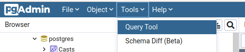
Open PGAdmin4 and connect to your local database, and open the Query Tool under the tools menu.
Lets start with something simple and show all the data we uploaded, to do this we will use the code:
SELECT * FROM public.da_boundary;
In this case the layer we added da_boundary and we can read this line of code as ‘Read everything from Stats Canada Boundary’.
And then press the Play button above the code editor.
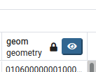
And you can go ahead and scroll to the geom column of the Data Output window, press the blue eye to view the map.