- 1. Introduction
- 2. Elevation
- 3. Contour Lines
- Creating a DEM
- 4. Comparing dataset quality
- 5. Hillshade
- 6. Creating 3D Scenes (This is where the computer will slow down)
- 3D Navigation
- Hypsometric tints
- 7. Fly through
- 8. Assignment 5 (5%) due before next weeks lab
1. Introduction
Technologically speaking, we are hoping for a smooth lab since we upgraded our computers a few years ago. With that said it is important to keep in mind that working with 3D data is inherently more computationally intensive; and when working inside of ‘scenes,’ operations will take longer to complete, and the software may be more unstable than normal. We have lots of time in lab today, save often, and if something doesn’t work quite right, stay calm and remember we are here to learn.
This is simply the reality of working with large files in real-time 3D.
When working on your homework, you have an extra incentive this week to complete it in lab as opposed to using Osmotar as the 3D performance is substantially higher on the local computers as opposed to on the remote desktop.
2. Elevation
Conceptually, we are exploring elevation today. To get an idea of what we’re dealing with, start by opening up ArcGIS Earth (consider it a better–and still free–version of Google Earth) and navigate to the UNBC campus. Click on the ruler icon in the top left corner, then click somewhere in the Agora courtyard. The pop-up box will show you the elevation of the point you clicked on. Now, click somewhere like the pond below campus. See how the elevation is lower? Now click somewhere near the bottom of the hill – same thing. Each pixel in ArcGIS Earth also contains its elevation, which is what allows us to get the 3D view if you right-click and hold to tilt your view of the landscape.
3. Contour Lines
We’re going to open an existing project to start today’s lab. Open ArcGIS Pro, then select ‘Open another project’ from the center-right column. Select L:\GEOG205\Lab06\smithers\Lab04.aprx.
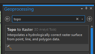
We’ll start by creating a Digital Elevation Model (DEM) from a contour layer. This is rarely necessary anymore as high quality DEM layers are widely available, but it is worth noting that it is possible to do so using the “Topo to Raster” tool using a contour layer as your input.
Creating a DEM
Open the Tools (Geoprocessing) pane from the Analysis tab
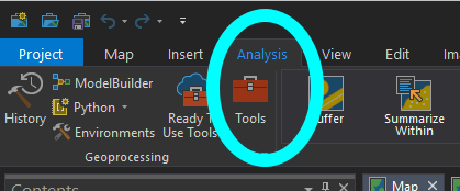
Search for the “Topo to Raster” tool
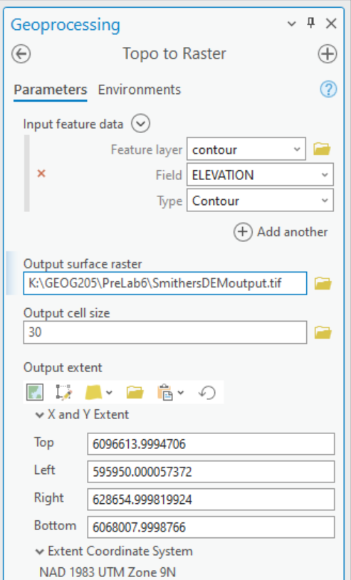
Set:
Feature Layer to ‘contour’
Field to ‘ELEVATION’
Type to ‘Contour’
For Output surface raster, MAKE SURE to change your save location to your K: drive, or the tool will not run.
Output cell size to ’30’
For output extent, click the tiny triangle next to the large yellow map sheet icon and choose ‘contour’ from the drop down (Note that the numbers in the boxes below will have updated, but otherwise it will look largely the same).
Leave all other settings as default and press run (This will take 1-2 minutes to complete)
Next, in your drawing order, turn off your contour contour layer.
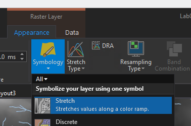
Select the new DEM layer you created, and set the symbology to stretch (Raster Layer > Symbology > Stretch). Turn off the vegetation layer.
You should have something as below:
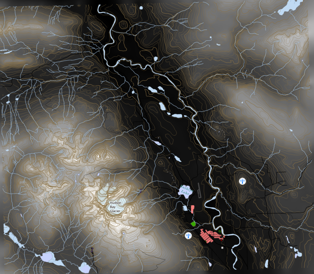
The pixels of this image represent the elevation, where white pixels are the highest values and therefore the highest elevation.
It is more common to receive elevation data as a DEM than as contours. Note that if you want to make a topographical map, you could produce the contours from the DEM with the “Contour” tool. We will not be doing this in today’s lab, but the process is very similar as above: pick the input DEM layer, give it an output name, and set the interval. This is also the best way to convert contours from Feet to Metres while still having even number, though note that this will reduce data quality due to interpolation.
A NOTE ABOUT SAVING AT THIS STAGE: You will not be able to save this project using the save icon at the top of the screen, since you are accessing this project file from the L: drive. Instead, go to Project > Save Project As, and select somewhere on your K: drive.
4. Comparing dataset quality
We now have a DEM that we created with 30 metre pixels based on a contour line dataset. Let’s compare it with a purpose-built DEM layer from the BC TRIM data.
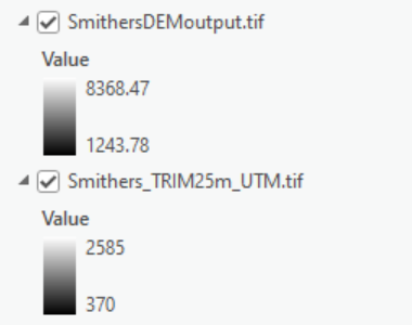
In the Catalog pane, add the L:\GEOG205\ folder as a new folder connection. Once added, open the Lab06 folder, then add ‘Smithers_TRIM25m_UTM.tif.’
As its name suggests, this DEM has 25 metre pixels. Drag this new layer down in the drawing order until it is right next to the DEM layer you created earlier. Turn off your vegetation and contour layers, and any other layers you feel are getting in the way. Now toggle whichever of the two DEM layers is above the other DEM, and notice the difference in resolution.
See how the DEM we created based on the contour lines appears softer? This lower resolution allows for less detail. You may also notice that the Values for each layer are different – this is because the contour layer we used was in feet rather than metres, and so our DEM is now also in feet.
5. Hillshade
Digital elevation models are not the most visually appealing on their own, so to add some visual style we will create a hillshade.
Create hillshade
Select one of your DEM layers. If you never altered the output it will be called TopoToR_cont1, or use the TRIM DEM.
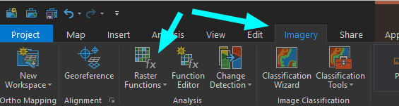
Open Imagery > Raster Functions
At the very bottom you will find Surface > Hillshade
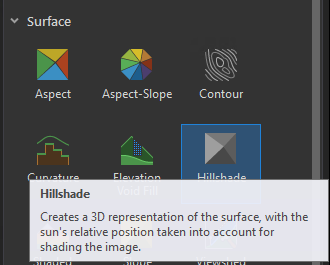
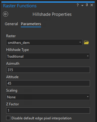
We will start by making a Traditional Hillshade:
Select your DEM created in previous step from the drop down, and leave type as traditional.
Azimuth is the compass direction the ‘sun’ will be coming from to cast shadows. 315 degrees represents North West. If you want your shadows on the other side of the mountain, this can be changed.
Altitude is how high on the horizon the ‘sun’ is in degrees with 0 being at the horizon (very strong shadows cast), and 90 being directly above (very few shadows, with no discernible direction).
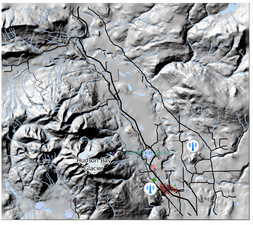
This should produce results as below. Toggle your contour layer on and off to see how the contour lines align with the hillshade.
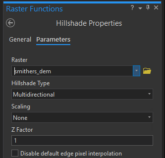
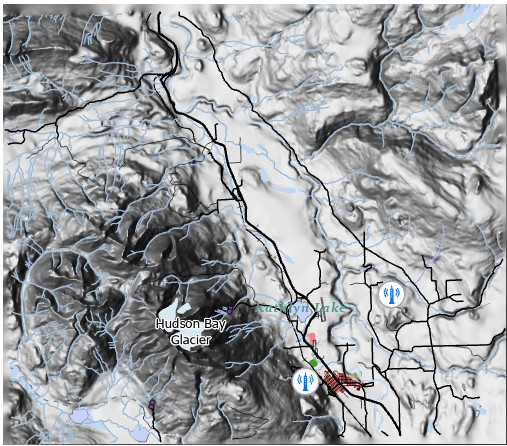
If you want to avoid shadows all being on one side of the terrain, instead of setting the Altitude to 90 degrees, use multidirectional as opposed to traditional hillshade.
Next, turn off the DEM layer, and all but one of the hillshade layers you just made
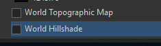
Ensure World Topographic Map and World Hillshade are turned off.
Move the hillshade layer you still have turned on to the very top of the Drawing Order.
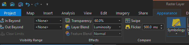
In the top ribbon, under Raster Layer, set Transparency to 60%, and Layer Blend to Luminosity.
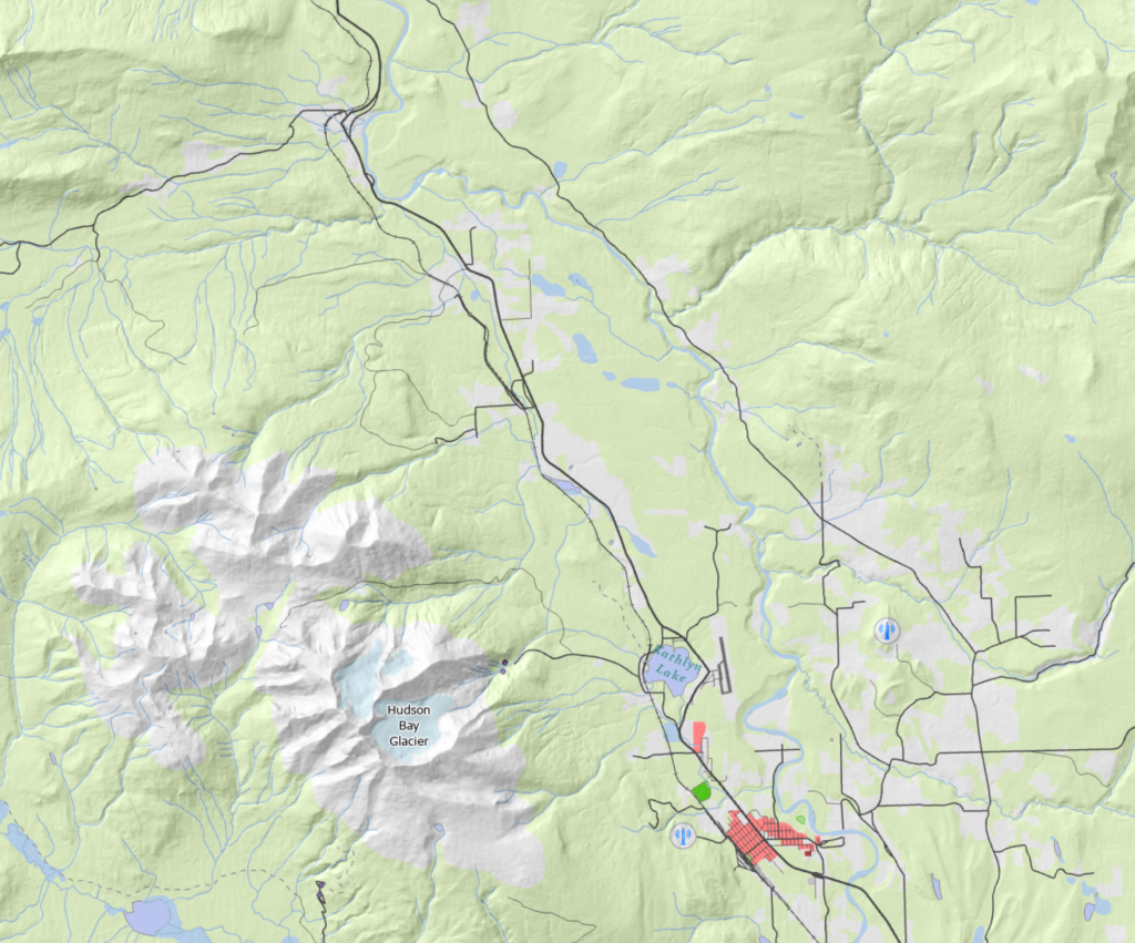
If you turn your vegetation layer back on, your map should now have a nice 2.5D effect. Go ahead and save your project, then close ArcGIS so we can start fresh.
6. Creating 3D Scenes (This is where the computer will slow down)
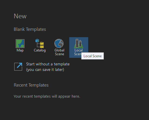
Open ArcGIS Pro again and instead of creating a new Map, create a new Local Scene from the templates and name your project something like lab06-3d.
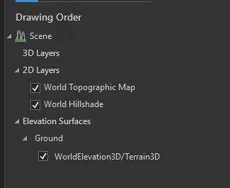
Now let’s examine the drawing order for the Scene. In the map we had only a single category, and now we have three categories.
3D Layers: this is for layers that have elevation information attached (i.e. contours). We will not be using any of these right now, these layers will be displayed at an altitude based on the contained data.
2D Layers: these are the layers you have been working with to date, and function exactly the same as they did in the map, except they will be draped over an Elevation Surface
Elevation Surfaces: this is the 3D data that 2D layers will be displayed against.
REMEMBER THIS: On 3D Layers, the elevation can either be above ground level or absolute. When elevation is absolute, errors in alignment between 3D Layers and the Elevation Surface could cause the layers to end up below the ground and thus not visible. This may happen when you get to the assignment!
We will start by turning off all 3 of the default layers, giving us a clean canvas to work with.
Add a folder connection for the Lab 6 data L:\GEOG205\lab06
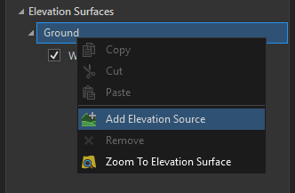
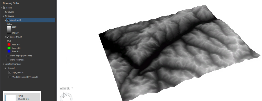
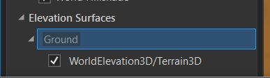
Right Click on Ground in the drawing order and Select Add Elevation Source. In the lab06 folder you will find an alps subfolder. Select the alps_dem.tif layer. Note that nothing in your Scene window will appear to have changed.
Next add the alps_ortho.tif file just as you would to any other map from the Catalog.
3D Navigation
You can use the 3D interface in the bottom left corner of the Scene window, which can be a little un-intuitive at first. You can also use the mouse movements below to control the map. Spend a couple of minutes exploring the alps and getting a feel for how to move the map around all of its axes.
Pan map – Left Click and drag
Zoom Map – Scroll Wheel or Right Click and Drag
3D Tilt – Middle Click and drag or [Shift] + Right Click and drag
Hypsometric tints
Note that the process for creating hypsometric tints is identical on the regular 2D Maps.
Start by adding alps_dem.tif as a visible layer in the 2D Layers section.
Next go into Imagery then Raster Functions
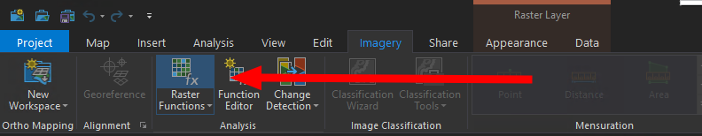
Search for “Shaded Relief”
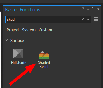
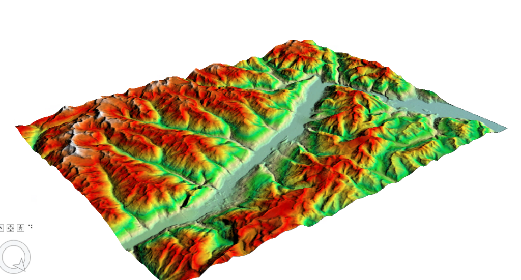
Set the Raster as alps_dem.tif, and pick a suitable Color Ramp: Note that Left to Right is low elevation to high elevation.
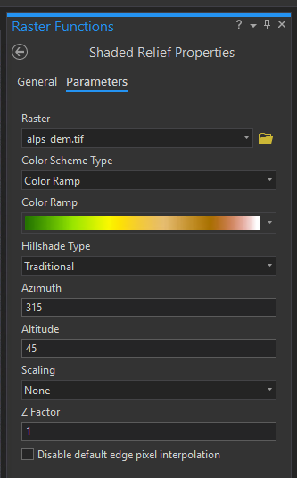
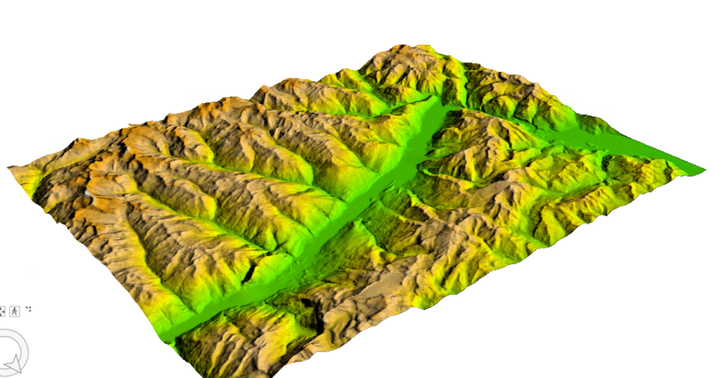
Do this process a couple more times with different colour ramps to see how the appearance changes. Note that different terrains will look better with different colour ramps.
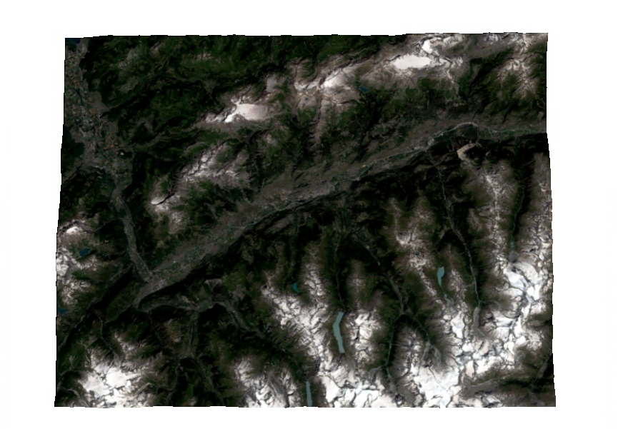
As a general note, ramps starting with a shade of blue are generally only appropriate when the scene contains water, in which case it should be adjusted so that the blue represents the waterline. As an example of this, take a look at the default colour ramp below. Aside from the red being overpowering, notice how if you did not know there was a settlement in the valley, this image makes it appear as though there is a river, and the tan looks like a beach-line. This is not helpful for your end users!
Note if your terrain looks too flat (or not flat enough) you can change the vertical exaggeration. Select Ground in the drawing order.
Then go into the Elevation Surface Layer tab and you will be able to set the Vertical Exaggeration.
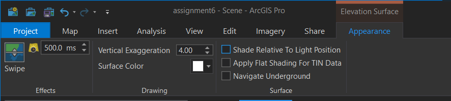
When you change the exaggeration, it will change the height of your map, and may take it out of your current point of view. The easiest way to find your map again is to right click on one of the layers you added and zoom to layer.
7. Fly through
At this point we have a 3D scene that we can look around, set to the perfect angle and send someone else a photo of, however in some cases, it may be more beneficial to send someone a video of this scene. We will accomplish this through a process known as keyframe animation.
Go to View and Add Animation
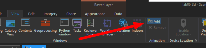
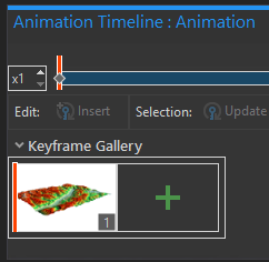
A new toolbar will have appeared below your scene with only a single button. First, adjust the view to how you would like your movie to start, then press “Create First Keyframe” and your Animation Timeline will appear.
Next move your view to a different angle you would like to show off, then press the Green +, and you will notice a 2nd frame.
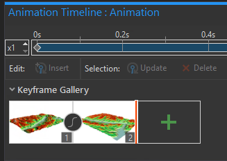
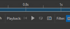
If you press the Play button, you will see the scene calculates all of the in-between frames to make an animation (though it will still be very choppy at this point).
You can continue adding as many frames as you like to create a tour of the scene.
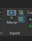
When the animation works the way you want it to, it can be exported as a movie. Exporting goes through a process called rendering. We will not be exporting the movie as part of lab as this process takes several minutes to an hour depending on the length of your animation. The time this process takes to complete is the reason why the preview was choppy, since the computer is unable to process frames of the movie as fast as it would need to in order to create smooth motion. The exported movies would play back smoothly and could be shared with clients or on social media.
8. Assignment 5 (5%) due before next weeks lab
For this weeks assignment, we will be building a simple map of Prince George. All of the layers you need are in L:\GEOG205\lab06\Assignment. You will be submitting two maps again this week.
Create a fresh new project file for your Lab 6 Assignment.
Part 1
1.) Make a simple map, using the Road Centerline, Trails, Building Outlines, and Hydrology, (you will also use Contours to build a DEM, but do not include the contour lines on your final map layout)
2.) Convert the Contour Layer into a DEM – Use 20m cell size (This will take about 4 minutes to process, a good time to stretch, or grab a coffee!)
3.) Create a hillshade From the DEM you just made
4.) Use the hillshade with some transparency to add the visual relief (Note: do not use the “shaded relief” tool, just the hillshade layer) like we did to make the 2.5D effect on the Smithers map at the beginning of lab.
5.) Create a Map Layout of this (remember the essentials like title, name, date, legend, etc.) and export it as a PDF to submit.
Part 2
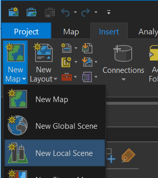
1.) Add a new local scene to your current project by going to Insert > New Map > New Local Scene
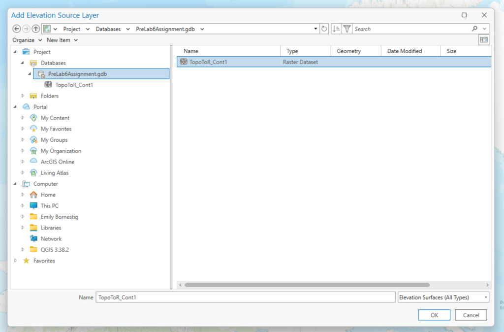
2) Replace the elevation surface with the DEM you created for the first map. You will find it inside of your projects default database once you go to add your Elevation Source Layer (refer back to the lab instructions to remember how to do this).
3) Add the layers for Roads, Trails, and Building footprints. Notice that your Building Outlines layer automatically gets sorted into the 3D Layers category. Remember what we talked about (*cough* in “Section 6. Creating 3D Scenes“) where elevation can be either at ground level or absolute? Right click on Building_Outlines > go to Properties > Elevation, then set Features are: from ‘At an absolute height’ to ‘On the ground.’ Allow your map to refresh (zoom in a bit if you want), and see if your building outlines show up.
4) Add a second copy of your DEM from Part 1 of the assignment, but this time put it in your 2D Layers. Set the Symbology to Stretch, and adjust the Raster Layer > Transparency to help show the changes in elevation.
5) Find an interesting viewpoint for your 3D map. You will most likely need to increase the vertical exaggeration (scroll up for a reminder how) as Prince George is relatively flat.
6) Change the base map to get a more pleasing appearance. DO NOT use any of the 3D Basemaps as they will override all of the layers you’ve added yourself, and we won’t be able to assess the work you did on the assignment. Try to avoid using base maps that have text on them, as the text will be distorted on the 3D surfaces. Alternatively, be creative with the viewpoint that you choose so that you minimize the amount of distorted text the end user can see.
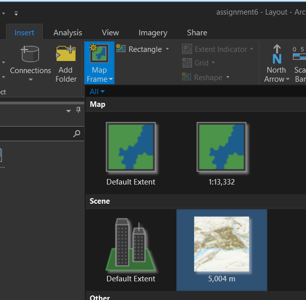
6) Create a new layout. Scenes can be added to layouts through the same process as we’ve done all semester.
7) Add your name and title. For the 3D scene, a legend is optional. Scale Bars and North Arrows should NOT be used as they will be incorrect due to perspective.
8) Export your map as a PDF.
Submit both maps to your TA through Moodle.