Build good habits now
A general reminder that GIS Software does crash, especially if we accidentally open files that are too large. Remember to save often, and if when the software crashes, it is not entirely unexpected. The most successful path forward will be to stay as calm as possible. Typically, GIS software will crash while working with particularly large or complex datasets. This can lead to a false sense of security as the software is stable when we have a low time investment, and will tend to crash after we have an hour of unsaved edits. Save often!
Adding Data to Our Maps
In today’s lab, we are going to explore the various kinds of data that we can add to our maps. Broadly speaking, this data comes in two main types that we’ve mentioned, but not explored in depth yet: Vectors and Rasters. Vectors come in Points (waypoints), Lines (roads or tracks from a GPS), and Polygons (outlines such as lakes or buildings). Rasters are imagery: this could be air photos or other data that has been rasterized. For example, the Lidar we used in the first lab started as point data and was rasterized into the digital elevation model we used.
Start a Project
As before, create a new project in ArcGIS Pro, and call it Lab3 (no spaces) inside of your GEOG205 folder (also no spaces) on your K: drive.
Use the catalog pane and add L:\GEOG205\lab03 as a folder connection.
Vector Data
Vector Data will be the primary source of data we will be using in this class and we will be looking at various ways of adding it. Our primary motivations for using vectors are that:
- Vector files generally occupy less storage space than raster files
- We have the ability to store metadata about individual vector features
- We get a great deal of control over how we symbolize vector data
Shapefiles
Shapefiles are an ageing file format but still can be thought of as industry standard as nearly all GIS software will open a shapefile.
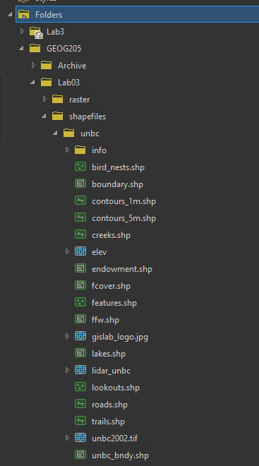
In the Catalogue pane of ArcGIS pro, take a look in L:\GEOG205\Lab03\shapefiles\unbc. You will see a variety of files listed. Note that we have one entry per file name. Now, open this same folder in the Windows file explorer: you will notice that there are in fact many more files here: a single shapefile is actually stored in multiple pieces.
Initially, you will probably see multiple files with the same names. In the View tab at the top of the file explorer ribbon, make sure the the box is ticked for ‘File name extensions’ in the ‘Show/hide’ section. Now you’ll be able to see the file extensions for all the files in the folder:
- .shp – File containing geometry
- .shx – Positional index of feature geometry
- .dbf – Contains attribute data for features
- .prj – File containing projection information (optional, but highly recommended)
- .sbn – Contains spatial indexes (optional file, but dramatically increases draw speed in large layers)
Inside of ArcGIS these are all presented as a single file, however, when interacting with shapefiles outside of ArcGIS, care needs to be taken to keep these files together, and if one is renamed, they must all be renamed with the exact same name.
Add the features.shp, roads.shp, and lakes.shp to your ArcGIS project from the Catalog pane.
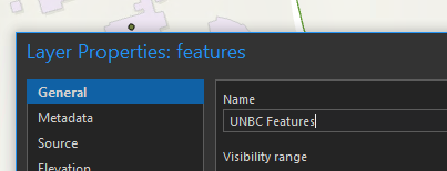
“Features” is a very generic name, so to help keep our table of contents clean, double click the Features layer in the drawing order panel and rename it to “UNBC Features”
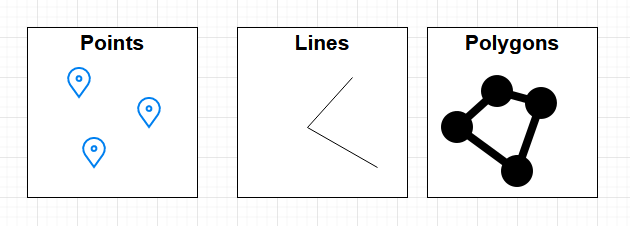
The (shapefile) data we just added comes in three types of geometry: points, lines, and polygons.
Each layer can only represent one single type of geometry. If we have a mixed dataset, such as rivers where large rivers are represented by polygons, and creeks as lines, we would either need two separate layers, or we would need to convert the geometry to be the same type for all features. An example of this conversion would be to buffer the small river lines to make them polygons, or to covert large river polygons to lines representing the banks (we saw an example of large rivers defined by lines in the rivers_093G layer that we used in Lab 02).
GPX
GPX or GPS Exchange format is a file type you may come across while working with data collected using handheld GPS Units. In comparison to Shapefiles, the GPX is a single file, and can contain all three geometry types at the same time (you will still only be able to load one geometry type per layer).
Despite this, ArcGIS Pro will not directly open these files in many cases (it will only load point features). For this reason, we will open another GIS software: QGIS.
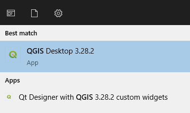
Once you have QGIS open, in the windows file explorer go to the folder L:\GEOG205\Lab03\gps_data and then drag and drop unbc_biodome.gpx onto QGIS.
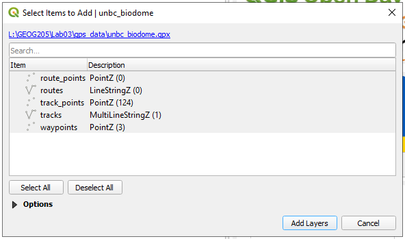
The dialogue presented shows the layers inside of the GPX files as well as the number of features in each layer in brackets at the end of each description. In this case, there is a track (recording of where the GPS was) represented as both a line (“MultiLineString” with 1 feature) and points (with 124 features), in addition to 3 waypoints. Click Select All, then Add Layers.
In QGIS you will see the lower-left corner has a layers pane that works much the same way as the Drawing Order in ArcGIS Pro. You can turn the layers on and off with the tick boxes to change what you see on the map.
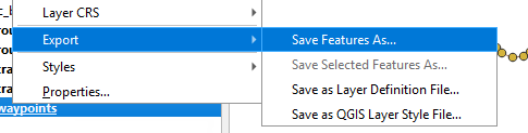
Right click on the waypoints layer > Export > Save Feature As
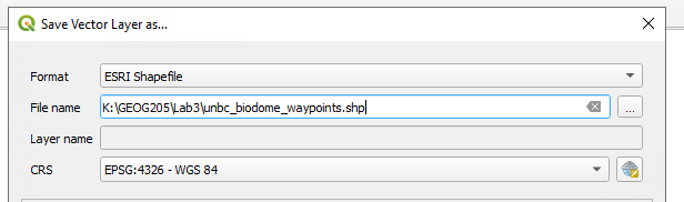
Set the Format to an ESRI Shapefile, and using the ellipsis (‘…’) button to the right of the File name, browse to your lab3 folder and save as unbc_biodome_waypoints.shp
Do the same for the track points and track line layers (toggle layers on and off to find the ones with data in them) and then add all three layers into ArcGIS Pro. Change the symbology of the waypoints layer (click on the point symbol below the file name) to differentiate the waypoints layer from the track points layer.
KML
KML stands for Keyhole Markup Language (KMZ is a compressed zip version of KML), and is the primary file type used by Google Earth. Due to the ease of access of Google Earth, KML / KMZ files are generally common in areas where data is produced without the need for a full GIS system. KML has an extra advantage over the other files we have looked at so far, in that they also contain a very basic amount of styling information in the form of line colour, and in the case of polygons, fill colour.
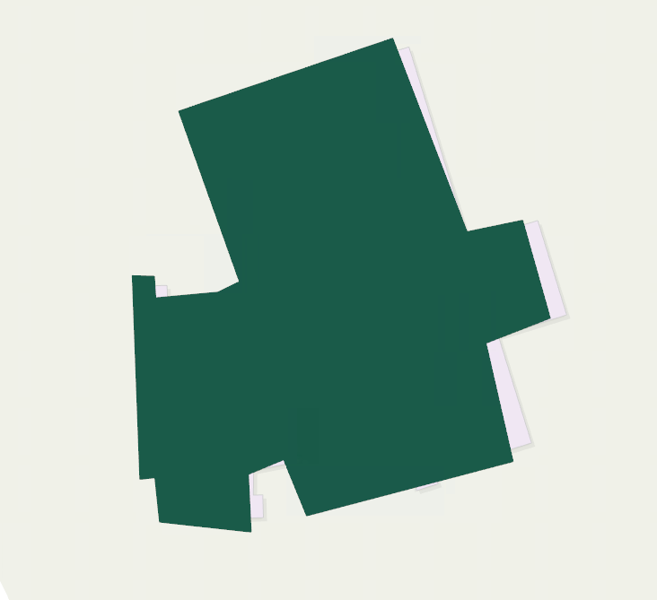
Add L:\GEOG205\Lab03\kml\Northern Sports Centre.kmz to your project and notice that the polygon automatically appears in UNBC’s Green.
Tabular Data
It is often common to get data in the form of spreadsheets. We are going to use a subset of a Canada-wide dataset from GeoNames. https://www.geonames.org/
If you wanted postal code data for all of Canada, you could find it on that website under Downloads > click on Free Postal Code Data > then download CA_full.csv.zip. You would find the file in your downloads folder, then extract the zip file into your Lab3 folder.
For today, copy CA_BC.txt from L:\GEOG205\Lab03, and paste in in your Lab3 folder.
Open Excel, select Open, then click Browse. Change the file type filter from ‘All Excel Files’ to ‘All Files.’
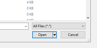
Navigate to and open the CA_BC.txt file you just extracted. You will be prompted with a dialogue to help Excel understand what type of data is contained within the file.
On the first page, make sure that the Original Data Type is set to Delimited, then proceed to Next.
On this page, we need to make sure the data preview looks like a spreadsheet. In this case, our Delimiter is a tab, and because there are some blank cells, we need to make sure ‘Treat consecutive delimiters as one’ is disabled so our data is not shifted after an empty column.
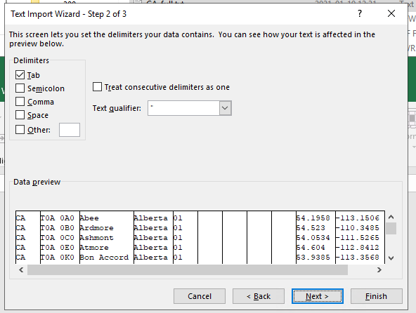
At this point you can click finish.
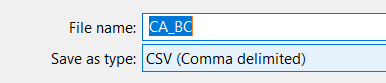
To help ArcGIS understand this data, we will click Save As, and save it as a CSV (Comma Separated Values) file. Essentially, we have just replaced Tabs with Commas in the file.
Now open this file in ArcGIS Pro. You may notice that it does not show up on the map, but rather at the bottom of the Drawing order as a “Standalone Table”. ArcGIS Pro knows it is a table, but does not know how to interpret the data yet. Right-click on CA_Full.csv in the drawing order and choose Open. The table will appear below the map. Scroll to the far right-hand side of the table and make note of which Fields (columns) contain the Longitude and Latitude – we will need this information in the next step.
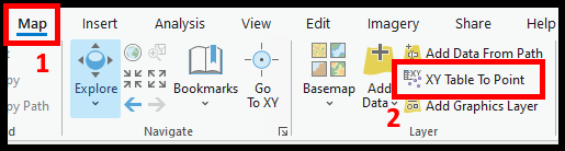
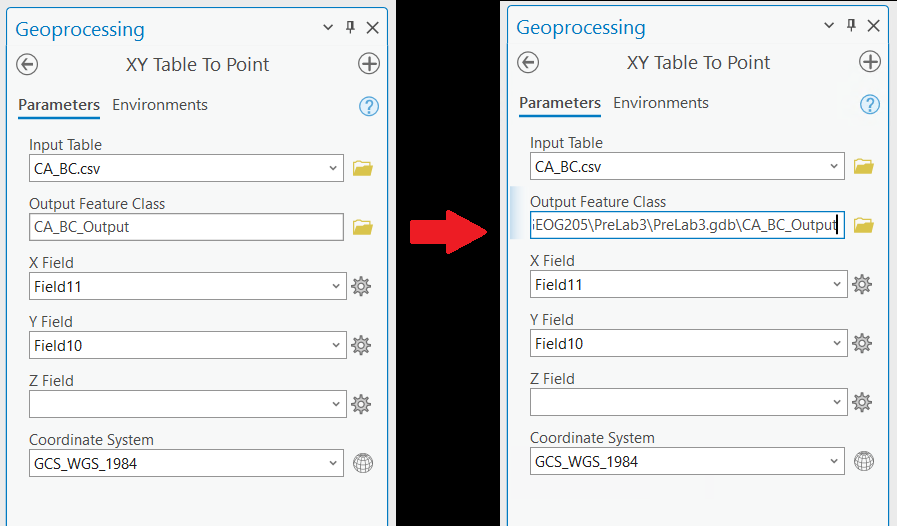
To make it show up on the map, we need to add XY Point Data using XY Table to Point.
We will then tell ArcGIS which Fields contain the positional data. Notice how clicking in the ‘Output Feature Class’ text box changes the contents to display the file path/storage location of the output. This is a great place to make sure that a) the file is going to be saved where you want it to be saved, and b) that there are no spaces in your file or folder names. If you want to change where the file gets saved to, click on the Folder icon at the end of the text box, and select a new save location and file name.
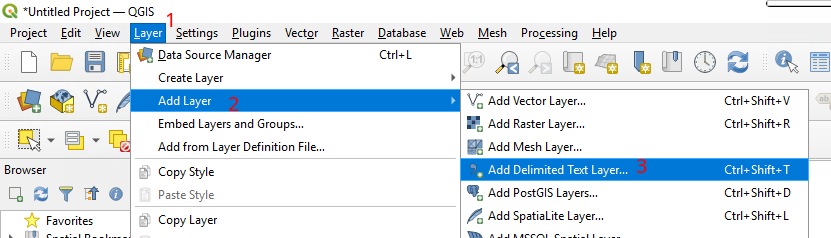
As an alternative, you could add the .txt file to QGIS directly following the steps in the image below, and then export it in the same way we converted the GPX File before. There is always more than one way to solve a problem!
Before Proceeding, right click on the Postal Code layers and remove them from your ArcGIS Pro project.
The postal codes CSV layer is relatively large and needs to be removed before proceeding.
Databases
The final form of vector input we will explore today is spatial databases. These range from file-based databases (Geodatabases, Spatialite) to Enterprise Database Management Systems DBMS (Such as Enterprise Geodatabase, PostgreSQL, MS-SQL with spatial extensions).
You have already been interacting with an Enterprise Geodatabase in this course when we use UNBC’s ArcGIS Portal. The ArcGIS Portal is storing all of its data in a PostgreSQL database; these systems are the highest performance option for storing data and provide the ability to work with large, rapidly changing data. Outside of the portal we also operate PostgreSQL servers on campus that store and serve TRIM, OpenStreetMap (entire globe), and BC Vegetation Resource Index, all data sources that exceed the file limitations of Shapefiles. That said, you are unlikely to come across such systems outside of large organizations or smaller businesses that focus specifically on geospatial data.
File-based geodatabases are the default method in which ArcGIS Pro stores data. In fact, if you look in the Catalog pane, you will find that there is already a lab3.gdb file in your lab3 folder. This is the geodatabase for your project, and anytime you export data it will be placed by default into this file. Inside of ArcGIS, a geodatabase looks a lot like a folder, but to the File Explorer in Windows, it is a single file. These are sometimes used to send someone multiple layers at once.
Rasters
The other broad category of data that you will run into is raster, which is likely more familiar to you when raster files are referred to as images. Common examples of this would be air photos, satellite imagery, scans of paper maps, and digital elevation models.
We added raster layers to our maps in both Lab 01 when we added the UNBC Campus orthoimage, and in Lab 02 when we added the scanned paper NTS map sheet. Today, we are going to look at a scenario you may run into if an image either doesn’t contain spatial information, or if this information is inaccurate.
Georeferencing
Two things before we begin:
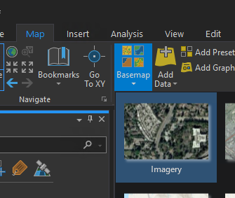
- Save your project, and
- Set the base map to Imagery so we have something to reference against:
In the File Explorer, copy L:\GEOG205\lab3\raster\campus20cm_2010.jpg to your lab 3 folder, and open the copy in ArcGIS Pro. Allow Arc to calculate statistics if it prompts you.
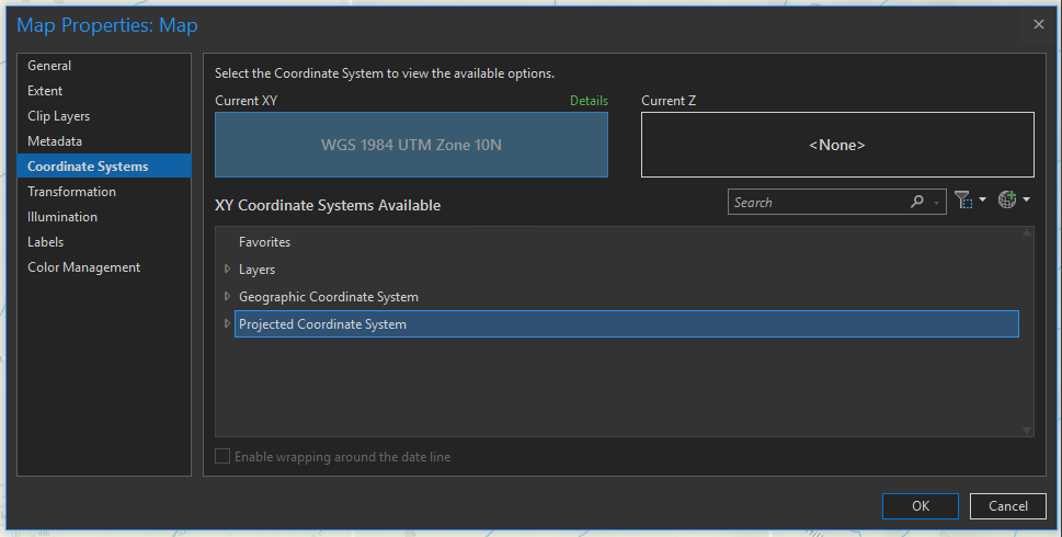
Make sure your Map is set to ‘WGS 1984 UTM Zone 10N’ by right-clicking on Map in the Contents pane, then Properties > Coordinate Systems, and verify the Current XY setting. If it is not correct you can find the projection under Projected Coordinate System > UTM > WGS 1984 > Northern Hemisphere > WGS 1984 UTM Zone 10N.
The data we added will probably appear in the middle of the Pacific Ocean. To make this show up where it is supposed to on a map, this image must be ‘georeferenced’.
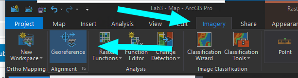
Select the ‘campus20cm_2010.jpg’ image in the drawing order, then go to Imagery in the top ribbon, then Georeference.
This is a tool that we can use to show ArcGIS Pro where the imagery belongs. You may also need to use this process if the data is only slightly misaligned.
This is done in a 2 step process:
- Prepare the data
- Adjust the data
- Note: If the image was only poorly referenced, but is relatively close to where it belongs, the preparation step could be skipped
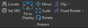
A great place to start is to zoom in on the campus on your basemap (World Imagery) layer, then press ‘fit to display’. This will cause the imported image to at least be in the general area of UNBC. You can then use the Move and Rotate tools to drag the image to the approximate location. Tip: Make sure the roads layer is still a) turned on and b) above the image in the drawing order so you can use it as a guide.
Adding Control Points
Next, we are going to add Control Points. Control points are created in pairs, first on the image we want to adjust (e.g., ‘campus20cm_2010.jpg’), and second on the target or what we want to match against (e.g., World Imagery). To make it easier to manage your control points, click “Control Point Table” in the Georeferencing Ribbon. This will open either a pop-up or an additional panel that will become very useful once we start adding control points. If it appears as a pop-up, click and drag the box until Arc will allow you to ‘dock’ it along the bottom of the window so that it remains accessible yet out of the way.
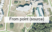
Make sure that the image we are georeferencing (“campus20cm_2010.jpg”) is on (box ticked) and active (highlighted in blue in the drawing order). Next, click on Add Control Points, either in the top ribbon or as an icon in the control point table toolbar. Your cursor should change to “From point (source)”, and an entry will be created in the control point table.
Zoom in on UNBC and click as close as possible to the center of the campus compass between the buildings.
At this point your cursor should change to “To point (target)”
Hide the image you are trying to adjust in the Drawing order and click on the same point on the basemap.
When you turn the image you are adjusting back on, you may notice it snap into place, however the image may still have the wrong rotation or scale. To fix this, we need to add more control points. Your cursor will default back to “From point (source)” after creating your first set of control points, but if it didn’t or you clicked on something else in between, go ahead and click “Add Control Points” again.
Create 4 more pairs of control points, following the guidelines below:
- Control points must be in the same place between images
- Control points should be spread apart and distributed across the image
- Control points should be at ground level whenever possible. Avoid trees, poles, and buildings as these can change with the camera perspective. If you must use these features, pick a point at their base.
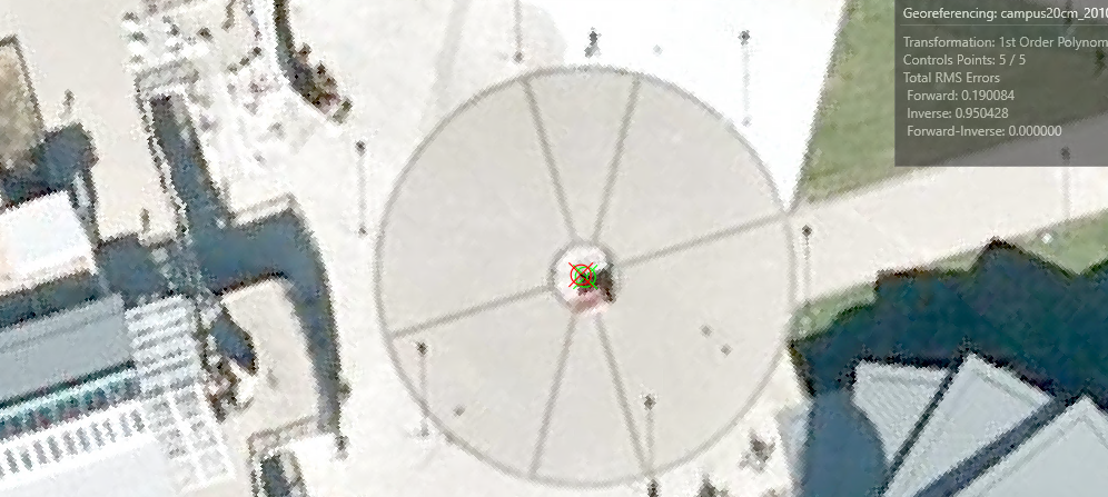
You should end up with something similar to this:
If you accidentally end up with control points that you don’t want to keep, you can manage them in the Control Point Table. Select the row of the points you wish to delete, then either tap the Delete key on the keyboard, or click ‘Delete Selected’. Notice that each pair of control points will turn turquoise on the map when you select them in the Table, so you can be sure you are deleting the correct points. If you really get mixed up, you can click the ‘Delete All’ button and start fresh.
Once you have at least 5 pairs of control points, notice how the road vector layer appears on top of the roads and lines up much better than it did before.
When you are happy with your results, select Save as New in the Georeference tab, then save your georeferenced image in your Lab 03 folder using the TIFF Output Format.
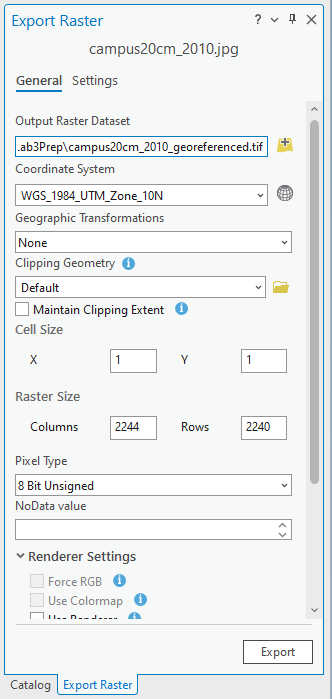
What will be exported is a GeoTiff, which is a Tiff file with coordinates in the metadata allowing this image to be opened in GIS software without the need to be georeferenced again.
Some potential sources of raster data might be:
PG Map: https://pgmap.princegeorge.ca/Html5Viewer/index.html?viewer=PGMap
If you are living outside of Prince George, your municipality may provide a similar service.
For Satellite images: https://earthexplorer.usgs.gov/
Editing Data
Something you will very quickly discover, if you haven’t already, is that spatial data often contains errors that need to be fixed before they are suitable for mapping. This can come in many forms such as missing data that needs to be added, anomalous data that needs to be removed, or data that just needs a little bit of an adjustment to better align with its precise location.
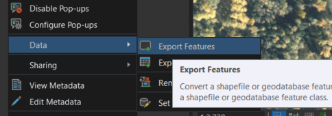
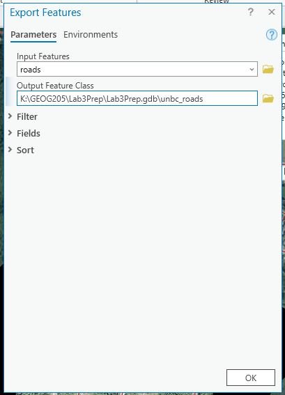
Never edit original data – it’s always good to be able to go back if you need to. Let’s make a copy of the roads layer: Right click > data > export features.
The only setting you should need to change is to rename your output file: Click in ‘Output Feature Class’ and notice where it is saving your file. At the end of the file path, after ‘[YourFileName].gdb\’, add your new file name – call it unbc_roads. By default, it will save into your project’s (Lab3) geodatabase.
For this next task, select your new roads layer and then the edit tab. Let’s start with a quick chat about the buttons available in the editor.
Selection tools:
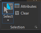
Before we can edit features, we need to select what we want to edit. There is a drop-down menu under Select for picking different selection tools when a rectangle selection is just not what you are looking for.
Attributes can be used to select features by values in the data table. For example, maybe you want to select all the creeks in a layer that have watercourse data. This is a feature that is better covered in GEOG 204 and GEOG 300.
Finally, there is a Clear button. It can be useful to always click this before selecting new features to make sure you are not editing features you have already finished with.
Clipboard:
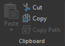
The tools in the clipboard section work pretty much as you would expect. It is somewhat unusual to paste within the same layer, however, one way to move features to a different layer is to cut, select the other layer in the drawing order, then paste.
Manage Edits:
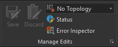
Here are two of the most important buttons: when we are finished editing, Save writes all the changes we made back to the original file. Discard is useful if you make a mistake that might have been too far back to undo actions all the way until you find the error, or you want to completely restart your edits. Discard will bring the layer back to the state it was in when you last clicked Save. On the topic of saving, save your project now.
Features:
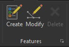
This is the last section of the top ribbon we are interested in. Both Create and Modify will open new panels on the right side of the screen, over top of the catalogue. Delete will simply remove whatever features are selected (selected features are displayed in turquoise, like we saw with the control points).
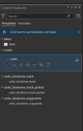
Create:
When the Create Features pane opens, it will show you a list of editable layers. Select the layer you wish to add features to, and you will be presented with a set of tools appropriate to the type of geometry (i.e., points, lines, or polygons) contained in that layer.
Take a few minutes to try out the various tools. Do not Apply/Save your edits, we will discard them before moving on. The idea here is to get a feel for how the tools work.
Snapping:
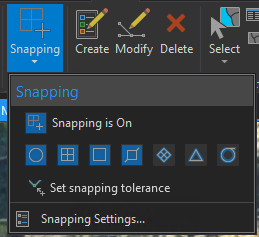
Snapping is useful when we want to make edits without gaps. Snapping will assign our cursor coordinates to exactly match nearby features. Try turning it on, and hover your cursor over a road feature. Does the cursor change to show what you are hovering on?
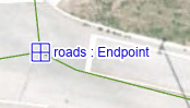
What happens if you hover over the middle of a line as opposed to the end?
Adding a road to the campus:
Make sure snapping is turned on, and add a road to the roads layer leading to the power plant on campus using the line tool, it should look like below. Double-click when you are done drawing your line. Ask your TA any questions you run into during this process.
Modify:
Modifying features is possibly the most finicky process in the class. It’s not hard, but mistakes are common and there is no shame in the discard button and starting over! Before we do this, if you’re happy with the current state of your project, save it, then try modifying features.
Let’s clean up the road in the bus loop to make it better match the background.
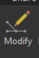
Click modify
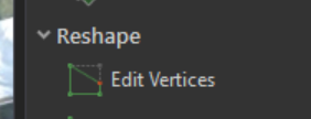
Then in the Modify Features panel that appeared on the right, find the Edit Vertices tool under Reshape in the panel on the right.
Then click on the road in the bus loop. Once selected, a new toolbar will appear at the bottom of the map.
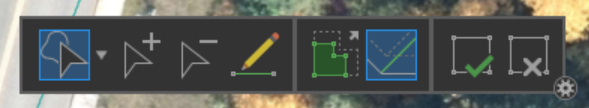
The first tool from left to right is the lasso selection tool, you can use the drop-down to pick a different selection tool if you prefer.
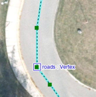
Draw a selection over several vertices, then hover over one of the selected vertices until your cursor changes to “roads: Vertex” at this point you can click to drag the nodes.
The next tool is the Add Vertex tool, with this tool selected you can click on a line segment to add a vertex at that point and then click and drag to make corrections.
Following that is the Remove Vertex tool, with this tool selected simply click on a vertex to remove it.
Finally in this section is the Continue Feature tool, this is much like the add vertex tool except instead of placing a vertex between existing vertices, clicking on the map will create a vertex and connect it to the most recently created vertex in the geometry.
Spend some time cleaning up the road and getting used to the tools.
Don’t forget if you make a mistake you can undo it with [Ctrl] + [z], or the back button in the upper left of ArcGIS Pro. Or, make use of the Cancel button at the end of the extra toolbar to undo all your recent edits.
Lab 3 Assignment
For this week’s lab, you will be making a map. Your map will consist of several layers that you will need to import into your project and edit. At a minimum, your map should also contain:
- Title
- Scale bar (with logical segments)
- Your name and the date
- Vector layers should be identifiable (ie. different colours and a legend) – if it’s not perfect, don’t worry, we are doing symbology next week!
- Disable any ArcGIS Pro basemap layers (e.g., World Imagery, World Hillshade, etc.)
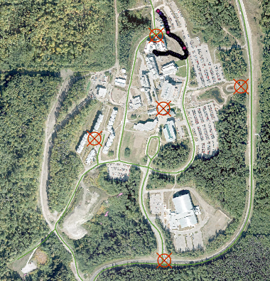
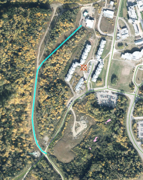
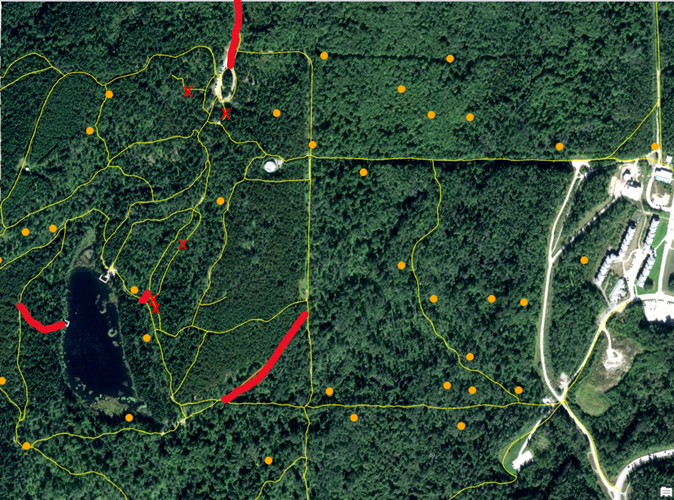
Your map will cover the trails near Shane Lake with an extent similar to the image below.
1. Add layers to the map
In the folder L:\GEOG205\Lab03\assignment_data you will find:
- unbc_pNeo_2021_RGB.tif
- trails shapefile layer: copy this to your K: drive from the L: drive as we will be editing it, and we don’t edit original data!
- If you do this in the file explorer, be sure to copy all the trails files, not just trails.shp
- Alternatively, add this vector layer from L: to your project via the Catalog pane in ArcGIS Pro, then use the dropdown (right-click on it in table of contents) and choose data-> export features and save this new shapefile in your lab folder on the K: drive. Then, remove the original shapefile from your project and use your saved copy.
- bird_nest.csv
2. Add the bird nest data as XY Point Data
Scroll back in the lab instructions for a reminder of how to do this! Remember that clicking on the coloured point, line, or rectangle beneath the layer you want to edit will open the Symbology pane that will allow you to change how the layer is displayed (click Apply once you make changes), and also remember that zooming in and out on your map will force the map to refresh and display changes you made. Style the bird nest points so that they have good contrast against the dark green of the forest.
3. Edit the trails layer
- Style the trails using a colour that provides good contrast against the raster layer.
- Remove 5 trails from your trail layer (see the image above for the trails marked with red X’s).
- Add 4 trails to your trail layer (see the bold red lines above for the ones to create); note that one of the trails is very short and can be hard to see – it is near the dock on Shane lake and near to the three trails we ask you to remove that are close to one another.
4. Create a new layer and add one more point
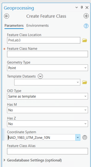
Part of working in GIS is locating, or sometimes creating, the data sets that you need. For this step, you’re going to create a brand new, empty shapefile, then add a new point to it to represent the water tower in Forests for the World (FFW).
To do this:
- Go to the Catalog pane in ArcGIS Pro, and right click on your Lab3 folder (the one with the house icon on it)
- Select New > Shapefile
- Assign a name to your layer in the ‘Feature Class Name’ box (something along the lines of ‘FFW_WaterTower)
- Set your Geometry Type (in this case, to ‘point’)
- Set the Coordinate System to the same coordinate system as unbc_pNeo_2021_RGB.tif by selecting that layer from the drop-down list.
- Click Run
Now that you have a new point layer in your Drawing Order, navigate the unbc_pNeo_2021_RGB.tif layer until you can see the round water tower near the parking lot for Forests for the World.
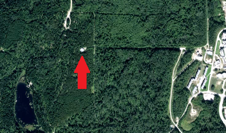
Select your FFW_WaterTower layer in the Drawing order, then go to Edit > Create, like we did earlier. Select Point under your FFW_WaterTower layer in the Create Features pane on the right, place your point on the map, then save your edits. Style your new point however you like, so long as it is adequately visible.
5. Create a new layout
Create a new layout in ArcGIS Pro, and make a Letter Sized, (ANSI) Landscape Orientation map. Make the extent of your map show all the bird nest points, and have the unbc_pNeo_2021_RGB.tif layer cover most if not all of your map frame. There is one bird nest that is right at the west edge of the raster layer, so do the best you can to minimize the amount of blank space in your map frame.
6. Add additional information to the map
Give your map a title, a scale bar, a legend (same way as you would add a scale bar – don’t worry about making it look nice, we’ll learn that next week!), your name, and the date.
7. Save your map as a PDF
Check out the Lab 01 instructions if you need a reminder of how to export your map from ArcGIS Pro. Submit the PDF file of your assignment to your TA via Moodle by the beginning of your next lab.