As a GIS Professional part of your job will be not only to analyze geospatial data but also to communicate your findings to end users. As time moves forward and data gets larger and larger simply producing maps and reports is no longer enough; allowing end users to interact with data directly is essential.
When looking at the models of data processing we have used to date, we have a server such as PostgreSQL, and a client QGIS, ArcGIS, FME, etc. When sharing data with other GIS Professionals they may have the appropriate software to share links to data sources directly however most people do not have GIS software on their system nor the knowledge of how to use such systems. To fill this gap we will be creating web clients that will sit between the server and the client to make the data more accessible.
For today’s lab, we will be creating our app in R deployed on a Shiny web server and using Leaflet as the mapping interface. Note that this is only one such possibility, there are a variety of Programming Languages, Webservers, and web mapping libraries that can be used in a variety of combinations. In our case, the purpose for choosing this is that we will be doing spatial statistics in R for the remainder of the course, and RStudio has graciously provided us with licensing for RStudio Connect which will allow for easy and reliable publishing of our apps.
Creating a Shiny App
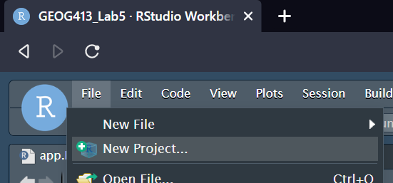
Start todays lab by logging into RStudio Workbench at https://rstudio.gis.unbc.ca and create a new project.
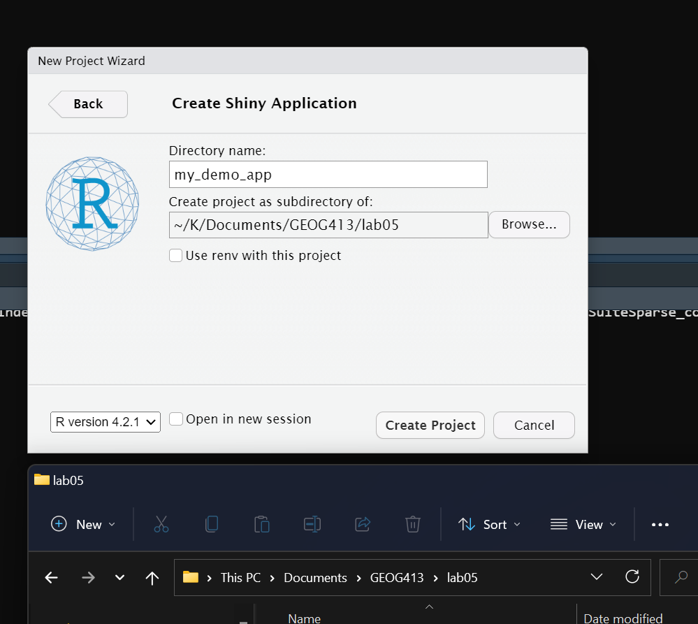
Create in a New Directory, and set type to Shiny Application.
The directory name is the name of your app, you may use whatever you like here, as to where to save it, Browse and put it somewhere inside of the K folder (this is your K drive)
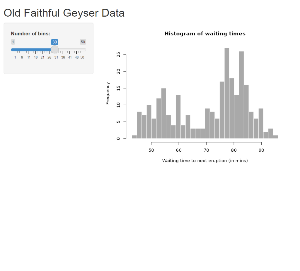
Once you press Create Project a demo app showing a histogram of the Old Faithful Geysers will be generated, we will modify this into our mapping project. First lets talk about the pieces of the app.
#
# This is a Shiny web application. You can run the application by clicking
# the 'Run App' button above.
#
# Find out more about building applications with Shiny here:
#
#    http://shiny.rstudio.com/
#

library(shiny)

# Define UI for application that draws a histogram
ui <- fluidPage(

    # Application title
    titlePanel("Old Faithful Geyser Data"),

    # Sidebar with a slider input for number of bins
    sidebarLayout(
        sidebarPanel(
            sliderInput("bins",
                        "Number of bins:",
                        min = 1,
                        max = 50,
                        value = 30)
        ),

        # Show a plot of the generated distribution
        mainPanel(
           plotOutput("distPlot")
        )
    )
)

# Define server logic required to draw a histogram
server <- function(input, output) {

    output$distPlot <- renderPlot({
        # generate bins based on input$bins from ui.R
        x    <- faithful[, 2]
        bins <- seq(min(x), max(x), length.out = input$bins + 1)

        # draw the histogram with the specified number of bins
        hist(x, breaks = bins, col = 'darkgray', border = 'white',
             xlab = 'Waiting time to next eruption (in mins)',
             main = 'Histogram of waiting times')
    })
}

# Run the application
shinyApp(ui = ui, server = server)
Line 10: This loads the shiny framework.
Lines 13-33: Defines a variable ui, this is the description of the user interface of the app.
Lines 36-48: Defines a function with an input and an output, this function called server is the what our app does.
Line 51: Tells R to run a shinyApp with the user interface and server function defined above.
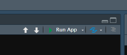
To run the app find the Run button at the upper right of the code window. Note if nothing shows up, you may need to enable pop-ups from the site to let it show.
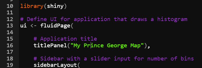
This template generated for us can now be modified to fit our purposes. Start with the easy option of changing the name of the app, in this case, we will be mapping the city of Prince George, you can change the title in line 16.
Using R to Create a Leaflet Map
Before R can create a leaflet map the leaflet library needs to be imported, the app will also make use of sf (simple features) and rgdal, you can go ahead and import them at the same time. Add these imports after library(shiny)
library(leaflet)
library(leaflet.extras)
library(sf)
library(rgdal)
next to show the map replace plotOutput() with leafletOutput(“map”), and remove the slider input.
# Define UI for application that draws a histogram
ui <- fluidPage(

    # Application title
    titlePanel("My Prince George Map"),

    # Sidebar with a slider input for number of bins
    sidebarLayout(
        sidebarPanel(

        ),

        # Show a plot of the generated distribution
        mainPanel(
          leafletOutput("map")
        )
    )
)
In the server section replace output$distplot with output$map as below
output$map <- renderLeaflet({
    m <- leaflet() %>%
      addTiles(group = "OSM") %>%
      setView(-122.75, 53.9, zoom = 11)
  })
Reload your app and you should see something like below
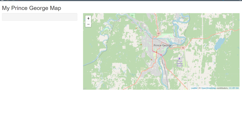
Inside the server block, a leaflet map called m was created with a tile group OSM, this is a predefined set of tiles that is a base map, as well as setting the view to zoom in to Prince George.
Before we proceed clean up the comments in the project as there is no longer a histogram.
#
# This is a Shiny web application. You can run the application by clicking
# the 'Run App' button above.
#
# Find out more about building applications with Shiny here:
#
#    http://shiny.rstudio.com/
#

library(shiny)
library(leaflet)
library(leaflet.extras)
library(sf)
library(rgdal)

# Define UI for application
ui <- fluidPage(

    # Application title
    titlePanel("My Prince George Map"),

    sidebarLayout(
        sidebarPanel(

        ),

        mainPanel(
          leafletOutput("map")
        )
    )
)

# Define server logic
server <- function(input, output) {

  output$map <- renderLeaflet({
    m <- leaflet() %>%
      addTiles(group = "OSM") %>%
      setView(-122.75, 53.9, zoom = 11)
  })
}

# Run the application
shinyApp(ui = ui, server = server)
A note on R functions
An interesting piece of syntax you should be familiar with is the pipe ( %>% ), pipes are often used to chain together functions rather than nesting inside of each other; this increases code readability.
You can also add more base layers to the map by adding more tile groups with the pip operator.
Try adding the following code
addTiles(group = "ESRI Topo", urlTemplate = 'https://server.arcgisonline.com/ArcGIS/rest/services/World_Topo_Map/MapServer/tile/{z}/{y}/{x}') %>%
      addTiles(group = "ESRI World Imagery", urlTemplate = 'https://server.arcgisonline.com/ArcGIS/rest/services/World_Imagery/MapServer/tile/{z}/{y}/{x}') %>%
      addLayersControl(
        baseGroups = c("OSM", "ESRI Topo", "ESRI World Imagery"),
        options = layersControlOptions(collapsed = FALSE)
      )
Actions in Shiny
Next we need to look at how to make interactive content in Shiny this is done by defining a trigger in the UI, and response to the event in the server.
The simplest form of Event will come from the use of a button, in it’s simplest form it looks like this in the ui
actionButton("do", "Click Me")and in the server (note this will print to the console, not to end users)
  observeEvent(input$do, {
    print('Thank you for clicking')
  })
Adding data to the map
First, the app needs to connect to a data source, in this case, there is a prince_george database on the PostgreSQL server we have been using. The connection (defined as the variable con) can be added right after your library imports.
library(RPostgres)
library(rpostgis)


db <- 'prince_george'  #provide the name of your db
host_db <- "pgadmin.gis.unbc.ca"
db_port <- '5432'  # or any other port specified by the DBA
db_user <- "sde"
db_password <- "unbc-user"
con <- dbConnect(RPostgres::Postgres(), dbname = db, host=host_db, port=db_port, user=db_user, password=db_password)
This con object can be used to run queries and send the results to R.
To add the data, reuse the button from before changing the action to trees and the text to ‘Add Trees’
Then in the server define an action to get the trees from the database and draw them on the map.
  observeEvent(input$trees, {
    results <- st_read(con, query = "SELECT * FROM trees") %>%
      st_transform(crs = 4326)
    addMarkers(leafletProxy('map'), data = results, group = 'trees', clusterOptions = markerClusterOptions())
  })
In this code when the server observes the event trees, it first reads data from the con, in this case, “SELECT * FROM trees”, and transforms to lat/lon. Then adds markers to the map; when adding to the map there is a few things happening here, leafletProxy() is a function that allows us to look up elements in the ui, as there is not a direct variable available, clusterOptions is used to combine the points to declutter the map; this is also important as drawing every marker is slow and makes the app feel unresponsive.
likewise you may want to remove markers this can be done by adding a button
actionButton(“remove_trees”, “Remove Trees”)
and an action
  observeEvent(input$remove_trees, {
     clearGroup(leafletProxy('map'), 'trees')

  })
Using the Bounding Box
At this stage, you may have noticed that you cannot zoom in far enough to separate all the trees, as such you may want to allow users to load unclustered data when zoomed in, this can be done with yet more actions. Start by adding a button for “individual trees”.
 observeEvent(input$individual_trees, {
    clearGroup(leafletProxy('map'), 'trees')
    bounding_box  <- input$map_bounds
    tree_subset <- paste0("SELECT geom FROM trees WHERE ST_Within(geom, ST_MakeEnvelope(",
                         bounding_box$east,", ", bounding_box$south,", ",  bounding_box$west,", ",  bounding_box$north, ", 4326))")
    print(tree_subset)
    results <- st_read(con, query = tree_subset) %>%
      st_transform(crs = 4326)
    addMarkers(leafletProxy('map'), data = results, group = 'trees')
  })
Recap displaying data
Before proceeding let us make sure everyone is on the same page, currently, the app code should look like this.
#
# This is a Shiny web application. You can run the application by clicking
# the 'Run App' button above.
#
# Find out more about building applications with Shiny here:
#
#    http://shiny.rstudio.com/
#

library(shiny)
library(leaflet)
library(leaflet.extras)
library(sf)
library(rgdal)
library(RPostgres)
library(rpostgis)


db <- 'prince_george'  #provide the name of your db
host_db <- "pgadmin.gis.unbc.ca"
db_port <- '5432'  # or any other port specified by the DBA
db_user <- "sde"
db_password <- "unbc-user"
con <- dbConnect(RPostgres::Postgres(), dbname = db, host=host_db, port=db_port, user=db_user, password=db_password)


# Define UI for application
ui <- fluidPage(

    # Application title
    titlePanel("My Prince George Map"),

    sidebarLayout(
        sidebarPanel(
          actionButton("trees", "Add Trees"),
          actionButton("remove_trees", "Remove Trees"),
          actionButton("individual_trees", "Individual Trees")
        ),

        mainPanel(
          leafletOutput("map")
        )
    )
)

# Define server logic
server <- function(input, output) {

  output$map <- renderLeaflet({
    m <- leaflet() %>%
      addTiles(group = "OSM") %>%
      setView(-122.75, 53.9, zoom = 11) %>%
      addTiles(group = "ESRI Topo", urlTemplate = 'https://server.arcgisonline.com/ArcGIS/rest/services/World_Topo_Map/MapServer/tile/{z}/{y}/{x}') %>%
      addTiles(group = "ESRI World Imagery", urlTemplate = 'https://server.arcgisonline.com/ArcGIS/rest/services/World_Imagery/MapServer/tile/{z}/{y}/{x}') %>%
      addLayersControl(
        baseGroups = c("OSM", "ESRI Topo", "ESRI World Imagery"),
        options = layersControlOptions(collapsed = FALSE)
      )
  })

  observeEvent(input$trees, {
    clearGroup(leafletProxy('map'), 'trees')
    results <- st_read(con, query = "SELECT geom FROM trees") %>%
      st_transform(crs = 4326)
    addMarkers(leafletProxy('map'), data = results, group = 'trees', clusterOptions = markerClusterOptions())
  })

  observeEvent(input$remove_trees, {
     clearGroup(leafletProxy('map'), 'trees')

  })

  observeEvent(input$individual_trees, {
    clearGroup(leafletProxy('map'), 'trees')
    bounding_box  <- input$map_bounds
    tree_subset <- paste0("SELECT geom FROM trees WHERE ST_Within(geom, ST_MakeEnvelope(",
                         bounding_box$east,", ", bounding_box$south,", ",  bounding_box$west,", ",  bounding_box$north, ", 4326))")
    print(tree_subset)
    results <- st_read(con, query = tree_subset) %>%
      st_transform(crs = 4326)
    addMarkers(leafletProxy('map'), data = results, group = 'trees')
  })

}

# Run the application
shinyApp(ui = ui, server = server)
Popups
Next, we will add some popups to our map, but before we can do this we need to understand some basic HTML (Hyper Text Markup Language). Essentially a Markup Language is a system of using special characters to define the structure of a text document within itself.
In HTML tags are used to control the structure, and have an opening tag <tag> and closing tag </tag>, everything inside of the tags fits into the tag’s structural element. There is also a handful of tags without closing such as <br> which defines a line break. To gain some practice in this go to https://codesandbox.io/s/xq2y4oyvo and start by deleting everything inside of the index.html file. Now try typing some text into the index file and you will notice it appears as plain text on the righthand side. As you can imagine at this stage to build a simple popup with only text we need not worry much about html; however we want more control.
Build a template for a popup for the tree points that shows the Tree ID, DBH, height, ages, and species of tree. If you are looking for ideas on tags there is a wonderful resource available here https://www.javatpoint.com/html-tags. Your final design should have each piece of information on its own line. As an example to get something like this
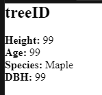
<h2>treeID</h2>
<br>
<b>Height:</b> 99
<br>
<b>Age:</b> 99
<br>
<b>Species:</b> Maple
<br>
<b>DBH:</b> 99
Moving the HTML into R.
With the popup designed the next stage will be to represent this in R, start by adding the library htmltools to your imports, then before the ui is defined create a variable called tree_popup. However when making this popup we will do something special adding a ~ after the = to make this a dependant variable; we will be using the past function to join all our text together. Start by adding the entire code from codesandbox.io as a string inside of the paste.
tree_popup = ~ paste()
tree_popup = ~ paste("<h2>treeID</h2>
<br>
<b>Height:</b> 99
<br>
<b>Age:</b> 99
<br>
<b>Species:</b> Maple
<br>
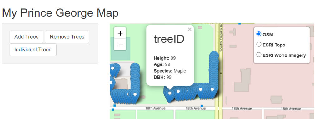
<b>DBH:</b> 99")Now to test the layout go to the observeEvent for individual trees and ass the paramater popup = tree_popup to the addMarkers command.
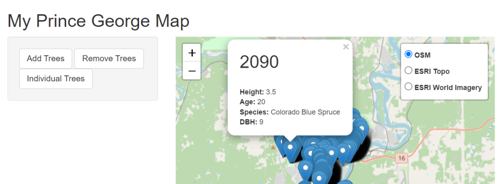
addMarkers(leafletProxy('map'), data = results, group = 'trees', popup = tree_popup)Now reload your application, zoom in, and press individual trees, finally click on one of the waypoints.
Then we got back to where the tree popup was defined and break the string into pieces. To break it simply close the quote add a comma and then restart the quote.
tree_popup = ~ paste("<h2>", "treeID", "</h2>
                       <br>
                       <b>Height:</b>", "99",
                     "<br>
                       <b>Age:</b>", "99",
                     "<br>
                       <b>Species:</b>", "Maple",
                     "<br>
                       <b>DBH:</b>", "99")
Finally as this is a dependant variable, replace the dummy values with the column names from the database
tree_popup = ~ paste("<h2>", objectid, "</h2>
                       <br>
                       <b>Height:</b>", treeheight,
                     "<br>
                       <b>Age:</b>", treeage,
                     "<br>
                       <b>Species:</b>", commonname,
                     "<br>
                       <b>DBH:</b>", dbh)
This should produce a result such as below.
Basic Spatial Operations
As a basic example of how you might manipulate the spatial data before display, let’s extend this example to show the distance the tree is from a traffic pole. To do this we will make use of the CROSS JOIN LATERAL to find the nearest traffic pole.
To build this takes the existing query you have from the observeEvent for individual trees, except the WHERE ST_Within piece to PG admin. Where you can build the query to answer the question.
SELECT geom, objectid, treeheight, treeage, commonname, dbh FROM trees
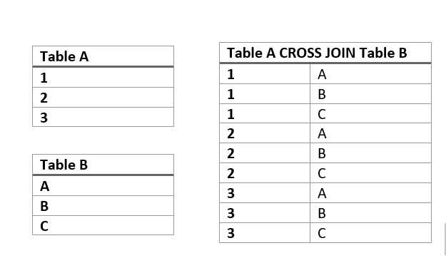
To get the distance to the traffic poles we will make use of the CROSS JOIN LATERAL, we are familiar with the word join, but have not yet seen the other words. First off a CROSS JOIN returns the cartesian product of two tables, that is every permeation.
One last piece of syntax we are adding is the PostGIS distance operator ‘<->’, combined with the Lateral join this allows us to join on an undefined distance (as opposed to using ST_D_Within().
And looks something like this
SELECT geom, objectid, treeheight, treeage, commonname, dbh, ROUND((ST_Transform(geom, 32610) <-> ST_Transform(geom_pole, 32610))::numeric, 1) AS dist, pole_id
FROM trees
CROSS JOIN LATERAL(
	SELECT traffic_pole.objectid as pole_id, traffic_pole.geom <-> trees.geom AS dist_deg, geom AS geom_pole
	FROM traffic_pole
	ORDER BY dist_deg ASC
	LIMIT 1
	) traffic_pole
It is very important to sort Ascending so the first result is the closest, and to LIMIT to 1, otherwise, we will get multiple rows for each tree. Put this new select statement back into your code, along with the pre-existing where clause. Finally, update the tree_popup to show this new data.
tree_popup = ~ paste("<h2>", objectid, "</h2>
                       <br>
                       <b>Height:</b>", treeheight,
                     "<br>
                       <b>Age:</b>", treeage,
                     "<br>
                       <b>Species:</b>", commonname,
                     "<br>
                       <b>DBH:</b>", dbh,
                     "<br>
                     <b>Closest Pole:</b>", pole_id, "is ", dist, "m away")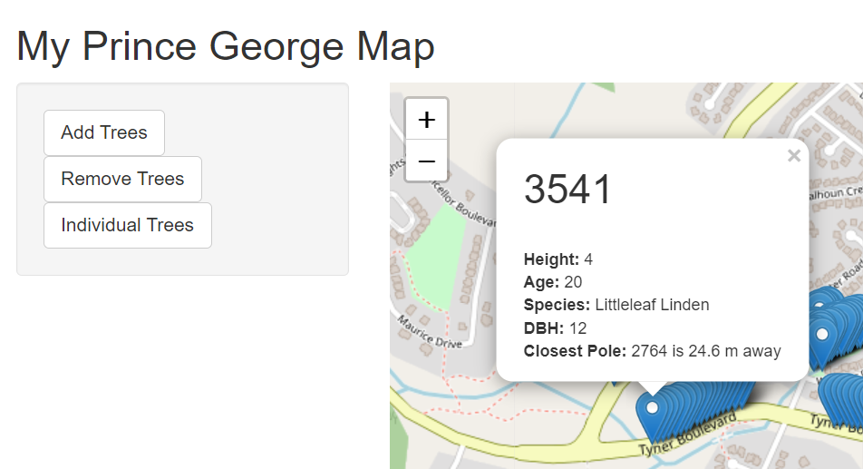
Putting Data into the database
One last thing before we finish up is to take a look at the pattern of how to put things into the database.
Add a text field to the input sidebarLayout
    sidebarLayout(
        sidebarPanel(
          actionButton("trees", "Add Trees"),
          actionButton("remove_trees", "Remove Trees"),
          actionButton("individual_trees", "Individual Trees"),
          textInput("name", "Name:", value = "", width = NULL, placeholder = NULL)
        ),
And a new event listener
  observeEvent(input$map_click, {
    print(input$map_click)
    coords = c(input$map_click$lng, input$map_click$lat)
    click_query = "INSERT INTO my_click (geom, name, time) VALUES (ST_MakePoint($1, $2), $3, $4)"
    print(click_query)
    q <- dbSendQuery(con, click_query, c(input$map_click$lng, input$map_click$lat, input$name, as.character(as.POSIXct(Sys.time()))))
    dbClearResult(q)
  })
This listener will do the action whenever the map is clicked on not a waypoint, and insert the contents of the text box to the name column.
You can see if it worked by checking out the demo app here https://connect.gis.unbc.ca/connect/#/apps/0018769b-3e06-48d2-90cc-f2379d731684/access
Publish your App
You can publish your app using the publish button
Add a new Publishing Account, choose “RStudio Connect” as the type. Servername is “connect.gis.unbc.ca” you can then login with your normal username and password.
Assignment
For this week’s assignment, you will make a demo app for a Realestate Agent, that can be used to find properties based upon their proximity to various services. These services will be
- Parks (park_open_space)
- Playgrounds (park_playground_equipment)
- Schools (school_property_status)
- Trails (trails)
- Bus Routes (transit_system)
- Fire Hydrants (water_hydrant)
Matt will provides skeleton code for UI tonight.
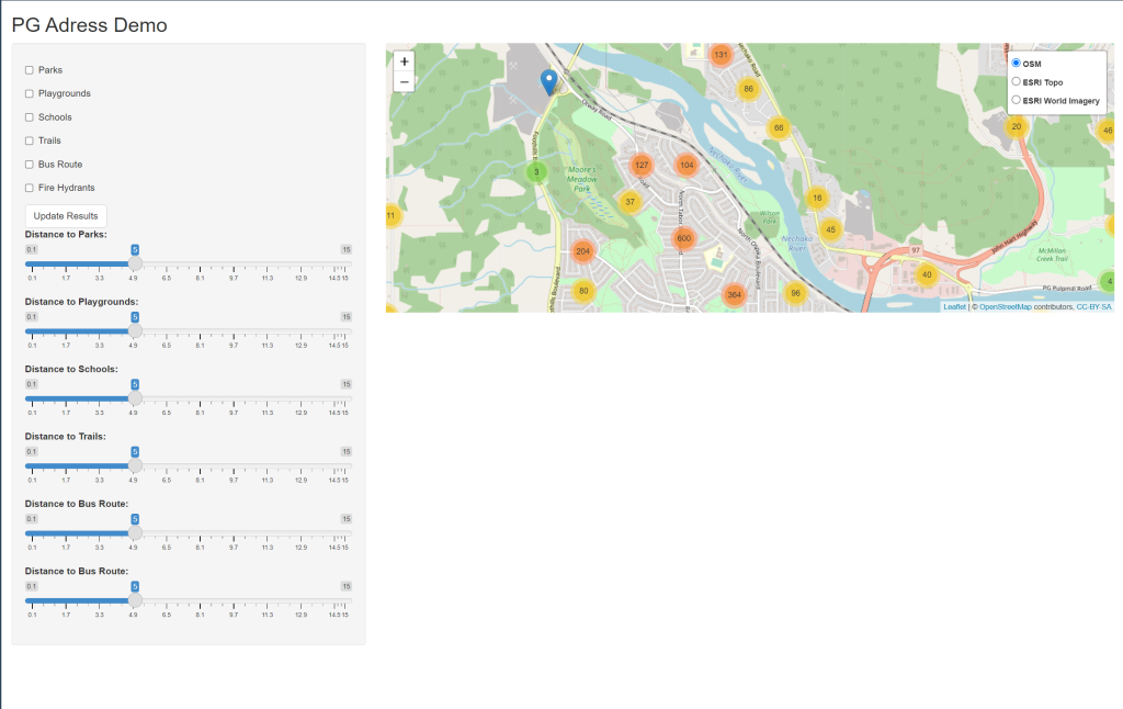
The app functions by showing properties within the specified distance for any categories that are turned on. Note that there is 6 cross joins, pressing update while all of Prince George is in view does run, but takes about 5-6 seconds to update, consider zooming in before pressing update results.
The assignment has 3 parts
- (2 marks) using the provided code anywhere ^^^^^ is present needs to be replaced with an alternate value to make the app work. And any comments #CHANGE ME should be replaced by descriptive comments.
2. (2.5 marks) extend the popups to show the distances to each category when the marker is clicked. (1.5 points for making a popup show all distances, 1 mark for applying style tags to give a visually appealing result. )
3. The CROSS JOIN’s run relatively slowly in this database, how might the database be altered to allow faster performance of this app?
Hints: For part one read any error messages in RStudio console. For part 2, design your popup outside of R, then do the value replacement as we did in lab.
library(^^^^^)
library(leaflet)
library(leaflet.extras)
library(sf)
library(rgdal)
library(RPostgres)
library(rpostgis)

db <- 'prince_george'  #provide the name of your db
host_db <- "pgadmin.gis.unbc.ca"
db_port <- '5432'  # or any other port specified by the DBA
db_user <- "sde"
db_password <- "unbc-user"
con <-
  dbConnect(
    RPostgres::Postgres(),
    dbname = db,
    host = host_db,
    port = db_port,
    user = db_user,
    password = db_password
  )

address_popup = ~ paste("<h2>", addrnumber, "</h2>")

ui <- fluidPage(# Application title
  titlePanel("PG Address Demo"),

  # Sidebar with a slider input for number of bins
  sidebarLayout(
    sidebarPanel(
      # Allow users to enable disance filters
      checkboxInput("park_enable", "Parks", value = 0),
      checkboxInput("playground_enable", "Playgrounds", value = 0),
      checkboxInput("school_enable", ^^^^^, value = 0),
      checkboxInput("trail_enable", "Trails", value = 0),
      checkboxInput(^^^^^, "Bus Route", value = 0),
      checkboxInput(^^^^^, "Fire Hydrants", value = 0),

      #CHANGE ME
      actionButton("update", "Update Results"),

      # Allow user to select distance in #CHANGE ME
      sliderInput(
        "park",
        "Distance to Parks:",
        min = 10,
        max = 2500,
        value = 5

      ),
      sliderInput(
        "playground",
        "Distance to Playgrounds:",
        min = 10,
        max = 2500,
        value = 5

      ),
      sliderInput(
        ^^^^^,
        "Distance to Schools:",
        min = 10,
        max = 2500,
        value = 5


      ),
      sliderInput(
        "trail",
        "Distance to Trails:",
        min = 10,
        max = 2500,
        value = 5

      ),
      sliderInput(
        "bus",
        ^^^^^,
        min = 10,
        max = 2500,
        value = 5
      ),
      sliderInput(
        "fire",
        "Distance to Fire Hydrant:",
        min = 10,
        max = 2500,
        value = 5
      ),
    ),
    mainPanel(leafletOutput("map"))
  ))

# Define server logic required to draw a histogram
server <- function(input, output) {
  output$map <- renderLeaflet({
    m <- leaflet() %>%
      addTiles(group = "OSM") %>%
      setView(-122.75, 53.9, zoom = 11) %>%
      addTiles(group = "ESRI Topo", urlTemplate = 'https://server.arcgisonline.com/ArcGIS/rest/services/World_Topo_Map/MapServer/tile/{z}/{y}/{x}') %>%
      addTiles(group = "ESRI World Imagery", urlTemplate = 'https://server.arcgisonline.com/ArcGIS/rest/services/World_Imagery/MapServer/tile/{z}/{y}/{x}') %>%
      addLayersControl(
        baseGroups = c("OSM", "ESRI Topo", "ESRI World Imagery"),
        options = layersControlOptions(collapsed = FALSE)
      )
  })

  observeEvent(input$^^^^^, {
    bb  <- input$map_bounds #CHANGE ME
    addr_query = paste0(
      "SELECT * FROM (
      SELECT addrnumber, geom,
      ROUND((ST_Transform(geom, 32610) <->
        ST_Transform(geom_park, 32610))::numeric, 1) AS dist_park, park_id,
      ROUND((ST_Transform(geom, 32610) <->
        ST_Transform(geom_playground, 32610))::numeric, 1) AS dist_playground, playground_id,
      ^^^^^
		^^^^^
      ROUND((ST_Transform(geom, 32610) <->
        ST_Transform(geom_trails, 32610))::numeric, 1) AS dist_trails, trails_id,
      ROUND((ST_Transform(geom, 32610) <->
        ST_Transform(geom_bus, 32610))::numeric, 1) AS dist_bus, bus_id,
      ROUND((ST_Transform(geom, 32610) <->
        ST_Transform(geom_fire, 32610))::numeric, 1) AS dist_fire, fire_id
      FROM civic_address_labels
      CROSS JOIN LATERAL(
        SELECT park_open_space.objectid as park_id,
          civic_address_labels.geom <-> park_open_space.geom AS dist_deg,
          geom AS geom_park
	      FROM park_open_space
	      ORDER BY dist_deg ASC
	      LIMIT 1) park
      CROSS JOIN LATERAL(
        SELECT park_playground_equipment.objectid as playground_id,
          civic_address_labels.geom <-> park_playground_equipment.geom AS dist_deg,
          geom AS geom_playground
	      FROM park_playground_equipment
	      ORDER BY dist_deg ASC
	      LIMIT 1) playground
      CROSS JOIN LATERAL(
        SELECT school_property_status.objectid as school_id,
          civic_address_labels.geom <-> school_property_status.geom AS dist_deg,
          geom AS geom_school
	      FROM school_property_status
	      ORDER BY dist_deg ASC
	      LIMIT 1) school
      CROSS JOIN LATERAL(
        SELECT trails.objectid as trails_id,
          civic_address_labels.geom <-> trails.geom AS dist_deg,
          geom AS geom_trails
	      FROM trails
	      ORDER BY dist_deg ASC
	      LIMIT 1) trails
      CROSS JOIN LATERAL(
        SELECT transit_system.objectid as bus_id,
          civic_address_labels.geom <-> transit_system.geom AS dist_deg,
          geom AS geom_bus
	      FROM transit_system
	      ORDER BY dist_deg ASC
	      LIMIT 1) bus
      CROSS JOIN LATERAL(
        SELECT water_hydrant.objectid as fire_id,
          civic_address_labels.geom <-> water_hydrant.geom AS dist_deg,
          geom AS geom_fire
	      FROM water_hydrant
	      ORDER BY dist_deg ASC
	      LIMIT 1) fire
      WHERE ST_^^^^^(geom, ST_MakeEnvelope(", bb$east, ", ", bb$south, ", ",
        bb$west, ", ", bb$north, ", 4326))) AS address_table
      WHERE TRUE") #WHERE TRUE allows every possible optoin to start with AND

    #CHANGE ME
    if (input$park_enable){
      addr_query <- paste(addr_query, "AND dist_park <=", input$park)
    }
    if (input$playground_enable){
      addr_query <- paste(addr_query, ^^^^^)
    }
    if (input$school_enable){
      addr_query <- paste(addr_query, "AND dist_school <=", input$school)
    }
	^^^^^
    ^^^^^
    ^^^^^
    if (input$bus_enable){
      addr_query <- paste(addr_query, "AND dist_bus <=", input$bus)
    }
    if (input$fire_enable){
      addr_query <- paste(addr_query, "AND dist_fire <=", input$fire)
    }

    clearGroup(leafletProxy('map'), 'addresses')
    results <- st_read(con, query = addr_query)
    #  st_transform(crs = 4326)
    addMarkers(
      leafletProxy('map'),
      data = results,
      group = ^^^^^,
      clusterOptions = markerClusterOptions(maxClusterRadius = 25),
      ^^^^^
    )
  })

}

# Run the application
shinyApp(ui = ui, server = server)