Lab 02 | RTK post-processing (PPK)

In recognition of the National Day of Mourning Sept 19th 2022, there will be no lab this week. The assignment is due before lab Sept 26th 2022, and if you have any requestions regarding this material or assignment reach out to Matt.

The following shows instructions specific to the Emlid GNSS, each manufacture will provide software for processing, file extensions may vary, but the theory behind what is happening will stay the same. At a high level the steps we are doing are:

1. Determine the Precise location of the base station.
2. Compare recorded data from base and rover, applying needed shifts from the now known base location to make an updated path of the rover.
3. Use the updated rover path to fix the location of recorded events (waypoints).

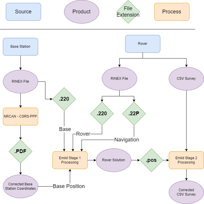
Working from the files collected the below diagram shows the flow of data to get to corrected GPS data. As many of the products are zip files containing multiple elements the green diamonds show the file inside the .zip that will be passed to the process.

If the process were to be completed without Precise Point Positioning (if we only needed relative position from base, as opposed to wanting to know exactly where on earth the base is the NRCAN processing can be omitted and the base position would be determined from the .22O file.

Another option would be to use a survey monument as opposed to PPP, in this case there are two options, the better option if you know the coordinates of the monument the base station is placed on, you would enter these into the base station when setting up, as it will then be useful for RTK while surveying, and again position will be filled from the .22O file. If for some reason you didn’t know the location at the time of the survey (perhaps you found it after arriving on site, set up on it, and looked up info after getting back to the office), the coordinates of the monument would be used in place of the CSRS-PPP coordinates.

We will now go through an example of some data collected in the summer, follow along to get a feel for the software, and then complete the assignment based on this weeks data.

Start by copying the entire contents of L:\GEOG413\lab02 into your K: drive, the software we are using (emlid studio) will write files inside the rover directory, as you do not have write permission to L: this process would fail if files are left in place.

Processing PPK Data

Log into Osmotar (https://gis.unbc.ca/support/remote-access-gis-servers/) note that Emlid Studio is not installed on the lab computers, however if you are in the lab you can always use Remote Desktop to connect to Osmotar.

We will work with the data in 01-06-2022 to start

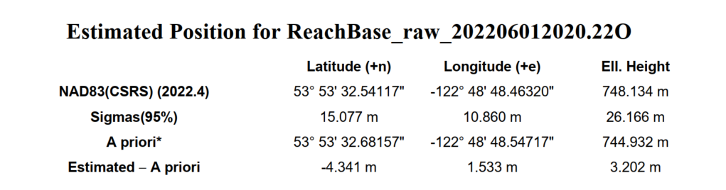
1. The first step of the process is to perform the PPP corrections for the base station, this has already been done for you, the results are in the file ReachBase_raw_202206012020.pdf. For your reference this is done by registering at https://webapp.csrs-scrs.nrcan-rncan.gc.ca/geod/tools-outils/ppp.php?locale=en uploading the entire RINXEX zip from the base station, and results will be e-mailed to you in 1 – 24 hours.
2. Open Emlid Studio (There is a shortcut in the lab02 folder, otherwise the program is in C:\Program Files\Emlid Studio\Emlid Studio.exe)

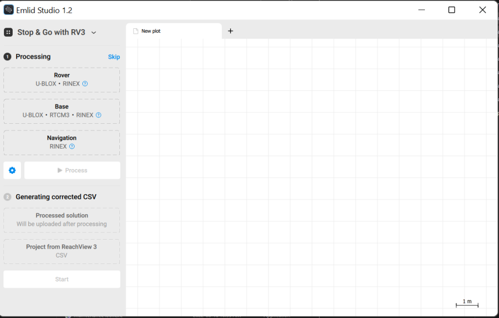
3. In the upper left corner, make sure the processing mode is set to “Stop & Go with RV3” this will provide the workflow we need for working with the outputs from the Reach View 3 App that we used in last weeks lab.

3.1 For Rover add the file ReachRover_raw_202206012020_RINEX_3_03\ReachRover_raw_202206012021.22O

3.2 For Base add the file Base_raw_202206012020_RINEX_3_03\ReachBase_raw_202206012020.22O, a drop down menu will have appeared defaulting to “RINEX Header Position” this is the pre PPP position of the base station, override this by picking “Lat/Lon/Height, dms” and entering the ‘A priori’ coordinates from ReachBase_raw_202206012020.pdf. Set the antenna height to 1.6m.

3.3 Navigation will be the .22P file from the rover: ReachRover_raw_202206012020_RINEX_3_03\ReachRover_raw_202206012021.22P

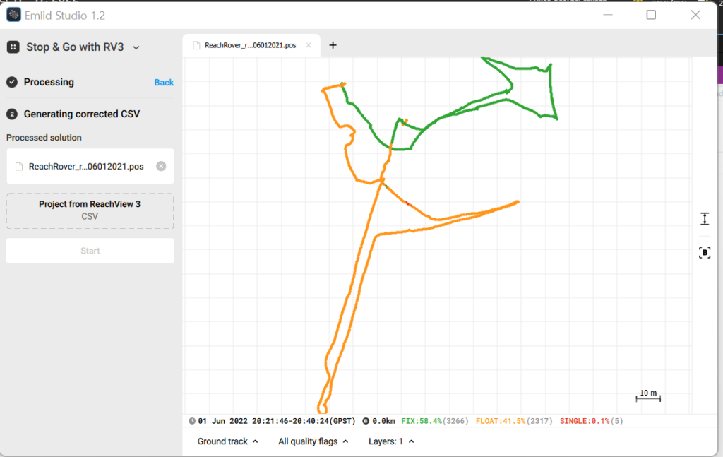
3.4 Press process and wait for the new .pos file to appear in the preview. This is a track of where the Rover was thought the survey.

4 Add ‘413 RTK SETUP1.csv’ as the project from ReachView 3 and press start.

The output will be found in the ReachRover_raw folder in the form of a .csv.

View the Results of PPK

Open QGIS and add both the survey and corrected servey.

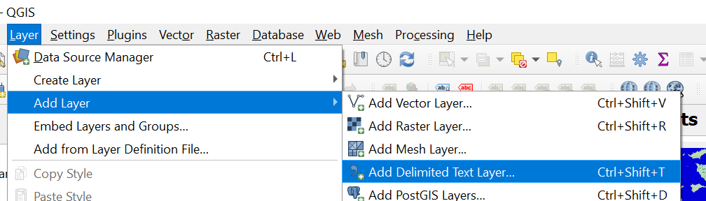
This can be done from the Layer Menu adding a Delimited Text Layer

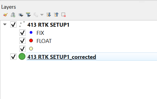
Optionally you may want to change the symbology to be more meaningful.

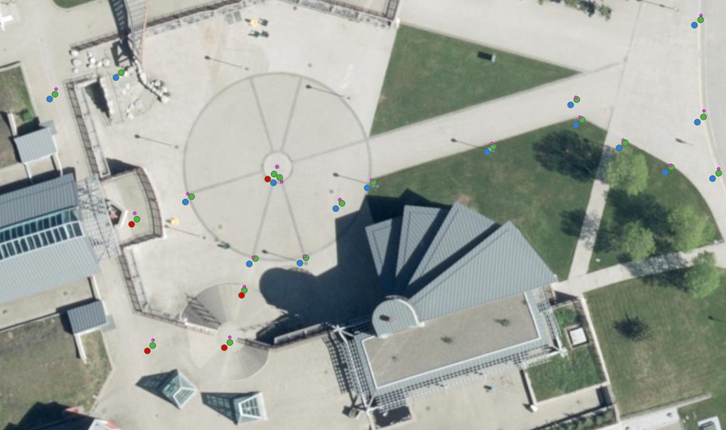
To demonstrate this I have also placed pink dots where on the image the rover was located. Something important to remember here; where the green (corrected) and pink points differ may be remaining error from the GNSS or it may be error from the orthophoto (this can be especially problematic around buildings as the images must be distorted to try and follow the geometry of the buildings.

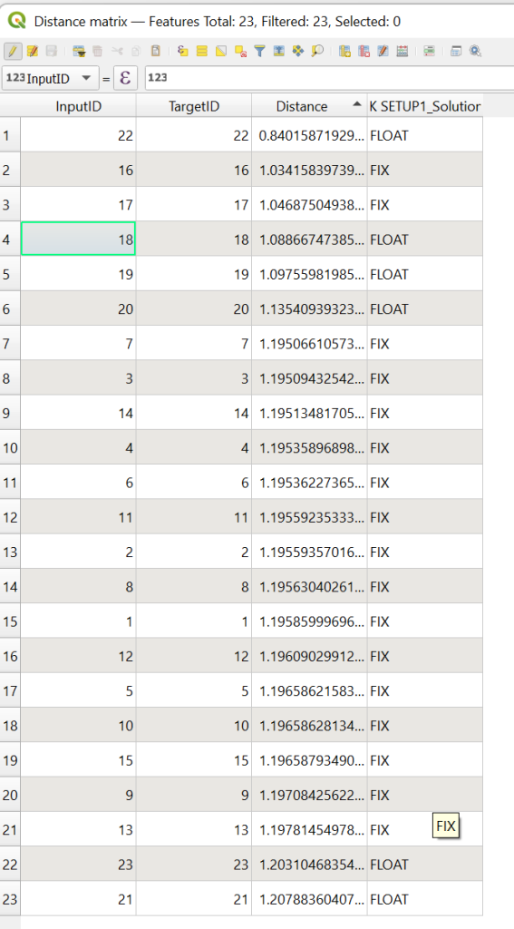
You can also optionally make a distance matrix to see how far the points have been shifted. (Vector -> Analysis -> Distance matrix)

Assignment

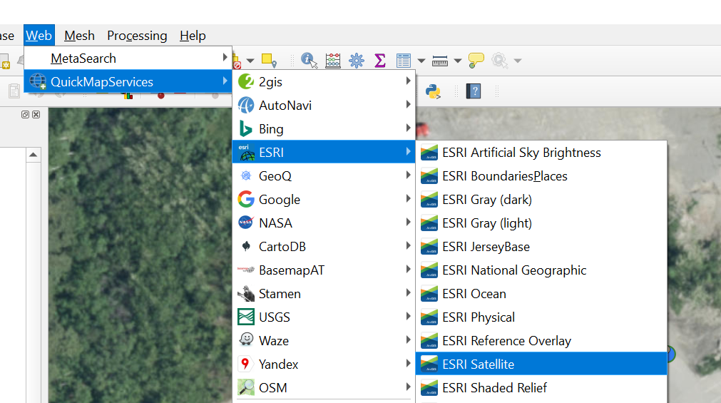
For this weeks assignment process the RTK data in lab02\13-09-2022, using 1.6m as the antenna height. After processing the data open it in QGIS with both the before and after, you can overlay it on a basemap buy using QuickMapServices (If QuickMapServices is not available you may need to install the plugin https://docs.qgis.org/3.22/en/docs/training_manual/qgis_plugins/fetching_plugins.html)

For your submission e-mail matt your corrected .CSV survey; along with the file answer the following questions.

Do you observe any pattern in the points in regards to weather they are a FIX or FLOAT solution?

Look at the point id 12, this point was captured with the rover touching the building, looking at where this point is on the map can you trust it? How does the PDOP (found in original CSV) compare to the average PDOP of the other points?