Review
Today’s lab is relatively short, before we begin we will do some interactive review of the lab material we have covered to date. Open the following link on one of the lab computers to follow along https://poll.gis.unbc.ca/p/31359493
Moran’s I
In today’s lab we will be looking at calculating Moran’s I, and Local Moran’s I using R; while in R we will also take a look at how we can produce reproducible reports using R-Markdown documents. For those unfamiliar Markdown is a tool used by various programs that allow for documents to be written in plain text, and rendered with various style options that were defined in said text.
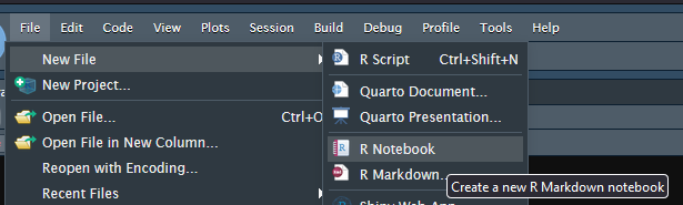
In RStudio you can create your first Markdown document by going into File, New and choosing R Notebook.
The main parts of the new new document are
- The heading starts and ends with —
- Markdown (Think of this as plain text
- R Code surrounded by “`
{r}“`
It is generally considered proper form to include your name and date in the file header.
---
title: "Morans-I"
author: "Matt McLean"
date: "07/11/2022"
output:
  html_notebook: default
  pdf_document: default
---
With that in place you can preview your document with the preview button

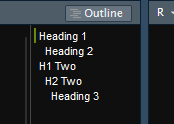
Finally the Table of Contents is another very helpful tool allowing the document to get some structure, outside of r code this is done with the # symbol, for example,
# Heading 1
## Heading 2
# H1 Two
## H2 Two
### Heading 3
Will produce the following headings, these will both appear in the final document, and can also be used for navigating within the document inside of R Studio, by clicking on the desired heading.
Preparing for Moran’s-I
For today’s lab we will be calculating Moran’s-I on some trials conducted by the Ministry of Forests, and will be using a package not normally available in R, this will be installed in the R command line with the following command.
install.packages('bcmapsdata', repos='https://bcgov.github.io/drat/')After this is installed you can import the libraries that we will be using today. Note there is an argument include=FALSE, this will prevent all these import statements from appearing in our final report.
```{r, include=FALSE}
library(bcdata)
library(bcmaps)
library(bcmapsdata)
library(tidyverse)
library(sf)
library(ggplot2)
library(ape)
library(units)
library(lubridate)
library(spdep)
library(sp)
library(tmap)
library(rgdal)
```
Download the trial data from GitHub https://github.com/FLNRO-Smithers-Research/OffSite_Trial_Reporting/blob/master/trial_data.Rdata
After you have downloaded into your working directory you can open with the following. It is relatively large code, as it expands the data from a single data-frame to multiple data-frames as well as calculate the extent of data (ie how many years does the data cover).
```{r}
load('trial_data.Rdata')

seedlots = all_data$seedlots
trees = all_data$trees
climate = all_data$climate
plots = all_data$plots
meta = all_data$meta
sites = distinct(select(merge(meta, plots, by="FID"), Location, FID, Lat, Lon), Location, FID, .keep_all = TRUE) #Location based on a plot not center of entire site
climate_sites = distinct(climate, ClimateStationID)
#List of years for which tree data is present, don't try to plot dates outside this range
years = year(as.character(min(as.Date(as.character(trees$Date))))):year(as.character(max(as.Date(as.character(trees$Date)))))
#List of years for climate data can differ from plot data.
climate_years = year(as.character(min(as.Date(as.character(climate$Date))))):year(as.character(max(as.Date(as.character(climate$Date)))))
#This function was used by many of the plots, moved here to not repeat
tree_summary=list()
for(year in years){
  tree_summary[[year]] <- trees %>%
    filter(year(as.character(Date)) == year) %>%
    # need to convert seedlot to factor
    mutate(Seedlot=factor(Seedlot)) %>%

    # Relevel condition factors
    mutate(Condition=fct_relevel(Condition,"Missing","Dead", "Moribund","Poor","Fair","Good")) %>% # reorder levels

    # Create plot summaries
    group_by(FID,Plot,Species,Seedlot,Condition) %>%
    summarise(n=n()) %>% # summarize number of trees at FID/Plot/Species/Condition
    ungroup()
}
```
To prepare for calculating the statistics the data must be opened, this sample data set contains 3 attributes that we can use to check for spatial auto correlation with Species, Seedlot (which tree farm are the seedlings from), and condition. You may note that there are also height and diameter columns, while potentially interested this data has been scrubbed from the open source side of the project.
attribute_list <- c('Species', 'Seedlot', 'Condition')Next the data needs to be sorted by trial site, (Identified by FID)
# Get list of unique trial sites
fids = as.data.frame(trees %>% distinct(FID) )
# Fore each trial site
for(id in 1:nrow(fids)) {
  # Convert iterator back to factor
  feature <- as.vector(fids$FID[[id]])
  # Select trees at trial site and that have a location
  tree_list = as.data.frame(trees %>% filter(FID == feature & (Lon != 0 | Lat != 0)))
  if (nrow(tree_list) > 0){
      # Print trial site name
      cat("  \n####",  as.character(feature), "  \n")
  }
  else{ # No trees were found in filter
    	cat("   \n", as.character(feature)", tree positions unknown")
  }
 }
To compute Moran’s I we need to convert the Trees to SF features and project into UTM
     tree_sf <- st_as_sf(tree_list, coords = c('Lat', 'Lon'))
     st_crs(tree_sf) <- 4326
     tree_utm <- st_transform(tree_sf, 32610)
Once the data is sf the next stage is to calculate the inverse distance of all points
	# Compute distance between points
    knn <- knn2nb(knearneigh(tree_utm))

    # Determine maximum Neighbor Distances
    all.linked<- max(unlist(nbdists(knn, tree_utm)))

    # Make Nerest Neighbor List
    tree_dist <- dnearneigh(tree_utm, 0, all.linked)

    # Style W is row-wise normalization
    lw <- nb2listw(tree_dist, style="W", zero.policy = T)
When working with categorical data it will be converted to factor in R, for proper calculation we would like this numbers to have a logical pattern, as such we will re-level the condition attribute
tree_list %>% mutate(Condition=fct_relevel(Condition,"Missing","Dead", "Moribund","Poor","Fair","Good"))
Finally we want to plot the attribute and calculate Moran’s I
    for (att in attribute_list){
      p <- ggplot(tree_utm) + geom_sf(aes(col = .data[[att]])) +
        coord_sf(datum = st_crs(tree_utm)) +
        theme(axis.text.x = element_text(angle = 45, vjust = 0.5)) +
        ggtitle(paste(feature, "-", att))
      print(p)

      # Test Morans I
      test <- moran.test(as.numeric(tree_utm[[att]]), lw)
      print(test)

      # Monty Carlo method
      MI <- moran.mc(as.numeric(tree_utm[[att]]), lw, nsim = 599, zero.policy = T)
      print(MI)

    }
This is put all together as the following function
attribute_list <- c('Species', 'Seedlot', 'Condition')

fids = as.data.frame(trees %>% distinct(FID) )
for(id in 1:nrow(fids)) {
  feature <- as.vector(fids$FID[[id]])
  tree_list = as.data.frame(trees %>% filter(FID == feature & (Lon != 0 | Lat != 0)))
  if (nrow(tree_list) > 0){
    cat("  \n####",  as.character(feature), "  \n")
    tree_sf <- st_as_sf(tree_list, coords = c('Lat', 'Lon'))
    st_crs(tree_sf) <- 4326
    tree_utm <- st_transform(tree_sf, 32610)

    # Compute distance between points
    knn <- knn2nb(knearneigh(tree_utm))

    # Determine maximum Neighbor Distances
    all.linked<- max(unlist(nbdists(knn, tree_utm)))

    # Make Nerest Neighbor List
    tree_dist <- dnearneigh(tree_utm, 0, all.linked)

    # Style W is row-wise normalization
    lw <- nb2listw(tree_dist, style="W", zero.policy = T)

    tree_list %>% mutate(Condition=fct_relevel(Condition,"Missing","Dead", "Moribund","Poor","Fair","Good"))


    for (att in attribute_list){
      p <- ggplot(tree_utm) + geom_sf(aes(col = .data[[att]])) +
        coord_sf(datum = st_crs(tree_utm)) +
        theme(axis.text.x = element_text(angle = 45, vjust = 0.5)) +
        ggtitle(paste(feature, "-", att))
      print(p)

      # Test Morans I
      test <- moran.test(as.numeric(tree_utm[[att]]), lw)
      print(test)

      # Monty Carlo method
      MI <- moran.mc(as.numeric(tree_utm[[att]]), lw, nsim = 599, zero.policy = T)
      print(MI)

    }


   }
   else{
     cat("   \nTree positions unknown")
   }
   cat("  \n")
}
Assignment
Create a Report on the Spatial Auto-correlation between Annual Precipitation and location of weather station using the stations data found in L:\GEOG413\lab08
You should be able to
- Import the data, and confirm the CRS / Translate if Needed
- Plot the data on a basemap (note that as you are making a PDF report interactive leaflet will not be an option)
- Report on if there is a correlation, and if it is significant.