A Visual Example
To start our exploration of PCA we will first look at the principal components of an image as it helps to intuitively show what the numbers mean, start by opening a Landsat image and plotting the image in R Studio.
# Load Libraries
library(raster)
library(dplyr)
library(imager)

# Open the image
# On windows path is 'L:/GEOG413....'
image = stretch(stack('~/L/GEOG413/lab06/prince_george_lc8.tif'))

#In landsat 8 images, red is band 4, green 3, and blue 2.
plotRGB(image, r = 4, g = 3, b = 2)

#plot all 7 bands.
plot(image)
At this point, you should be able to see an image of Prince George in 7 different wavelengths as captured by Landsat 8. Before the image can have the PCA calculated it must be converted to a data frame with only 2 dimensions (currently we have x, y, and band, we need xy, and band).
dim(image)
image.df <- as.data.frame(image)
dim(image.df)
If your dimensions are reduced you can now compute the Principal Components of the image using the dplyr library
pca <- prcomp(image.df)
and look at both a summary of the results, as well as the eigenvalues produced.
summary(pca)
pca
First take a look at the output of the summary
Importance of components:
                           PC1     PC2     PC3     PC4     PC5     PC6     PC7
Standard deviation     27.5248 21.8380 6.90914 2.79606 1.64263 1.05053 0.60443
Proportion of Variance  0.5854  0.3685 0.03688 0.00604 0.00208 0.00085 0.00028
Cumulative Proportion   0.5854  0.9539 0.99074 0.99678 0.99887 0.99972 1.00000
In this table we can see there are 7 principal components across the top (why are there 7?). They are shown along with the Standard Deviation of pixel intensities, the Proportion of Variance represented, and the Cumulative Proportion of variance. This is telling us, that Principal Component 1 represents 0.5854 of the variation in pixel intensities, and combined with Principal Component 2 this is 0.9539% of the variation.
Next, to understand what is happening we will look at the eigen vectors
Standard deviations (1, .., p=7):
[1] 27.5247652 21.8379751  6.9091408  2.7960560  1.6426283  1.0505273  0.6044305

Rotation (n x k) = (7 x 7):
                          PC1         PC2         PC3          PC4         PC5         PC6          PC7
prince_george_lc8_1 0.2740264 -0.35393469  0.24672391 -0.625697864  0.06229739 -0.05387918 -0.583511215
prince_george_lc8_2 0.2773480 -0.35022900  0.22127703 -0.298588252  0.04854514 -0.22025609  0.781939843
prince_george_lc8_3 0.3511632 -0.30326703  0.19843505  0.337055897 -0.69829000  0.37771787 -0.038087634
prince_george_lc8_4 0.3604207 -0.37716566  0.01484489  0.607506489  0.52145955 -0.24084764 -0.169206504
prince_george_lc8_5 0.5994954  0.71170044  0.35011765 -0.000371049  0.10429454  0.02400220  0.007198983
prince_george_lc8_6 0.4066549  0.07406538 -0.72124920 -0.095773666 -0.31641847 -0.44413104 -0.048991043
prince_george_lc8_7 0.2645867 -0.07643204 -0.45583349 -0.165842375  0.35104902  0.74167205  0.124704801
This table is showing a matrix of each band of input, along with each Principal component, the vectors provided here allow for conversion between the bands and the Eigen channels, showing how much weight each input has on the channel and vice versa.
For example, the eigenvectors are stored in the $rotation variable inside the PCA object, we can reconstruct band 6 with the following code.
image.pca <- pca$x
image$pc1 <- image.pca[,1]
image$pc2 <- image.pca[,2]
image$pc3 <- image.pca[,3]
image$pc4 <- image.pca[,4]
image$pc5 <- image.pca[,5]
image$pc6 <- image.pca[,6]
image$pc7 <- image.pca[,7]


plot(image$pc1, axes = FALSE)
plot(image$pc2, axes = FALSE)
plot(image$pc3, axes = FALSE)
plot(image$pc4, axes = FALSE)
plot(image$pc5, axes = FALSE)
plot(image$pc6, axes = FALSE)
plot(image$pc7, axes = FALSE)

pca$rotation[1, 1]

band  =  6
plot((image$pc1 * pca$rotation[band, 1] + image$pc2 * pca$rotation[band, 2] + image$pc3 * pca$rotation[band, 3] +
        image$pc4 * pca$rotation[band, 4] + image$pc5 * pca$rotation[band, 5] + image$pc6 * pca$rotation[band, 6] +
        image$pc7 * pca$rotation[band, 7] ))
Though we could also get back 99.07% of band 6 with this code
band  =  6
plot((image$pc1 * pca$rotation[band, 1] + image$pc2 * pca$rotation[band, 2] + image$pc3 * pca$rotation[band, 3]))
Some R Basics
R makes performing the PCA very simple however before getting back to PCA we will take some time to look at a couple of very popular packages in R, and the merge function.
The first is dplyr, the same library used for prcomp. Specifically a look at how data manipulation works. What is dplyr? According to their website:
dplyr is a grammar of data manipulation, providing a consistent set of verbs that help you solve the most common data manipulation challenges
https://dplyr.tidyverse.org/
This library is a common place to start data manipulation. Start by opening the ‘starwars’ dataset. It was added to your R environment upon calling library(dplyr). To see what is inside just type starwars.
starwars
work through the examples on https://dplyr.tidyverse.org/
The next package to look at is ggplot2 https://ggplot2.tidyverse.org/. here what is important to understand is that each plot is made of geometry and an aesthetic (aes) at a minimum. And may also contain, themes, facets, or other modifiers.
As an example of some plots we can use the built in cars dataset.
To make a scatter plot you could
ggplot(cars) + geom_point(aes(x = speed, y = dist, fill = speed))
The important parts of this are ggplot(data_set), then a geometry is added, in this case geom_point. Finally an aesthetic is added, most important here is defining the x, and y columns.
To make this a histogram you would simply change the geometry type
ggplot(cars) + geom_histogram(aes(x = dist))
Changing the appearance of the plot is as simple as adding a theme
ggplot(cars) + geom_histogram(aes(x = dist)) + theme_void()
If one of the handfuls of themes doesn’t provide what you are looking for there is also extra themes available.
library(ggthemes)
ggplot(cars) + geom_histogram(aes(x = dist)) + theme_economist()
Finally, let’s look at how to load and merge spatial data.
Start by opening some energy use / economic data for Canadian provinces from a CSV file, and opening a matching shapefile using the SF library.
energy_data <- read.csv('~/L/GEOG413/lab06/energy_data.csv')

library(sf)
province <- read_sf(dsn = '~/L/GEOG413/lab06', layer = 'pr_boundaries')
Now you can use the merge function much like a JOIN in SQL
province_energy <- merge(x = province, y = energy_data, by.x = 'prname', by.y = 'PRNAME')
Had the column names actually matched we could have used by = ‘colname’, instead of specifying x and y separately.
Back to PCA
Before we calculated PCA using prcomp(), now we will look at to to perform PCA step by step.
Make sure your data is open
# Open energy data CSV
energy_data <- read.csv('~/L/GEOG413/lab06/energy_data.csv')

# Use columns 2-8, (everything except province names)
pca_energy <- energy_data[,c(2,3,4,5,6,7,8)]

#Set row names to province names (we do not want to do statistics on the province names
rownames(pca_energy) <- energy_data$PRNAME
pca_energy
next define two functions, one to center the data, and another to scale the data
#standardize the data (center and scale)
center <- function(v){v-mean(v)}
scale <- function(v){v/sd(v)}

pca_energy.centered <- apply(pca_energy, MARGIN = 2, FUN = center)
pca_energy.scaled <- apply(pca_energy.centered, MARGIN = 2, FUN = scale)
Finally, calculate the PCA
#calculate covariance and eigen values
pca_energy.eigen <- eigen(cov(pca_energy.scaled))

pca_energy.eigen$values
Equivalently you could use the prcomp function
energy_prcomp <- prcomp(pca_energy, center = TRUE, scale = TRUE)
Next we want to make scree plots to help determine how important each factor is. To do this we need the cumulative sum of variance.
#calculate the proportion of variance explained by each component
pca_energy.ve <- pca_energy.eigen$values/sum(pca_energy.eigen$values)
pca_energy.ve
Usin par() to define multiple columns you can place plots side by side
par(mfrow = c(1,2), mar = c(4,5,3,1))
plot(pca_energy.ve,
     xlab = "Principal Component",
     ylab = "Proportion of Variance Explained",
     ylim = c(0,1),
     type = 'b',
     main = 'Scree plot')

plot(cumsum(pca_energy.ve),
     xlab = "Principal Component",
     ylab = "Cumulative Proportion of\nVariance Explained",
     ylim = c(0,1),
     type = 'b',
     main = 'Scree plot')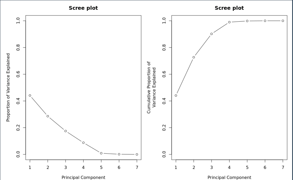
# Based on scree plot bend, pick first two PCA
pca_energy.loading <- pca_energy.eigen$vectors[,1:5]

#label the columns and rows
colnames(pca_energy.loading) <- c('PC1','PC2', 'PC3', 'PC4', 'PC5')
rownames(pca_energy.loading) <- colnames(pca_energy)
pca_energy.loading
# Score is matrix multiplication of COL's 1-4 by PC channels 1 & 2 pca_energy.scores <- as.matrix(pca_energy) %*% as.matrix(pca_energy.loading) # Set rownames to DAUID to allow merging tables rownames(pca_energy.scores) <- rownames(pca_energy) # Print livelihood scores pca_energy.scores
Plot your results
# JOIN da and PCA channels
province_pca <- merge(x = province, y = pca_energy.scores, by.x = 'prname', by.y = 'row.names')

#ggplot PC1
ggplot(province_pca) + geom_sf(aes(fill = PC1))
In the above notice that y is merged on row.names, think of this as a meta-column, as there is no column with the row names stored, however, we set the names while loading data so they could be referred to at this stage.
library(leaflet)
#Leaflet Plot
pal <- colorNumeric(
  palette = "Blues",
  domain = province_pca$PC1)

# NAD 1983 Albers Canada https://epsg.io/102001
epsg102001 <- leafletCRS(crsClass = "L.Proj.CRS", code = "EPSG:102001",
                       proj4def = "+proj=aea +lat_0=40 +lon_0=-96 +lat_1=50 +lat_2=70 +x_0=0 +y_0=0 +datum=NAD83 +units=m +no_defs +type=crs",
                       resolutions = 2^(13:-1), # 8192 down to 0.5
                       origin = c(0, 0)
)

web_mercator <- province_pca %>% st_transform(4326)
leaflet(province_pca, options = leafletOptions(worldCopyJump = F, crs = epsg102001))  %>%
  addProviderTiles("CartoDB.Positron") %>%
  addPolygons(color = ~pal(PC1))
To get a better sense what we are looking at print (pca_energy.loading), take a look at what is driving PC2,
#ggplot
library(gridExtra)
pc2 <- ggplot(province_pca) + geom_sf(aes(fill = PC2))
population <- ggplot(province_energy) + geom_sf(aes(fill = population))
demand <- ggplot(province_energy) + geom_sf(aes(fill = demand))
percapa <- ggplot(province_energy) + geom_sf(aes(fill = percapa))

grid.arrange(pc2, population, demand, percapa)
Finally, a quick look at the leaflet to make the map interactive.
Assignment
The assignment is worth 5 marks and due before lab on October 31st.
For this assignment, you will be calculated the PCA of a livability index based on four factors from the census, (Education -Secondary…, Education – Postsecondary…., Labour – Did not work, Labout – Worked). The data is available in the L drive with the data table post_college.csv, and the geometry censu_da_subset/bc_da_2016.shp.
Completing the code is worth 3 marks, additional questions are below.
# Open post_college census data, and select the columns of interest
livelihood_data <-

# Standardize the data (center and scale)

pca_livelihood.centered <-
pca_livelihood.scaled <-

# Calculate covariance and eigen values
pca_livelihood.eigen <-

# Calculate the cumulative proportion of variance for each component
pca_livelihood.ve <-

# Display above results in scree plots


# Based on scree plots how many PCA channels are significant?
# Puth these channels into the variable below, and name the rows and columns
pca_livelihood.loading  <-

# Use Matrix Multiplication to create the PCA channels
pca_livelihood.scores <-

# Set rownames to DAUID to allow merging tables
rownames(pca_livelihood.scores) <- rownames(pca_livelihood)

# Print livelihood scores
pca_livelihood.scores

# Use cencus boundaries as simple feature, plot with ggplot2
library(sf)
library(ggplot2)
library(leaflet)

# Filter data on load to avoid kernel crash, filter provided below.
da <- read_sf(dsn = '~/L/GEOG413/lab06/censu_da_subset', layer = 'bc_da_2016') %>%
  filter(DAUID %in% livelihood_data$COL0)

# JOIN da and PCA channels
da_pca <-

#ggplot PC1 and PC2


#Leaflet Plot PC1 and PC2
- How much variance is described by PC1?
- What input column is the primary driver of PC2?
- How much variance is described by the first 3 Principal Component Channels?
- What does PC represent?