For today’s lab, we will be expanding upon the skills for PostgreSQL and performing analysis inside the database using the PostGIS Extensions.

PostGIS has already been installed into the database you are using for this course, on a new database adding the extensions requires superuser privileges and is accomplished with the command
CREATE EXTENSION postgis;
Installing the PostGIS extension add several features to databases broadly this can be seen
- New data types: Columns can now have the data types of geometry or geography
- Spatial Functions: Typically these can be identified with the prefix ST_, and provide a variety of operations you are used to using in desktop GIS, such as area calculations with ST_AREA, computing buffers with ST_BUFFER, and many more, a complete listing is available in the documentation here: https://postgis.net/docs/reference.html
Adding Data to the database
For today’s lab, we will start by adding a large amount of data to the database, to accommodate a large number of records in the database we will be using FME Workbench to add data to the database. For those unfamiliar FME also known as the Feature Manipulation Engine, is a program produced by SAFE Software in British Columbia. The workbench works by creating a graph of dataflow starting with ‘readers’ then ‘transformers’ are applied, and finally ‘writers’ are used to output the manipulated data. FME is particularly well suited to processing large quantities of data from one format to another. While you could add the data using QGIS as we did last week it would take substantially longer for the process to complete.
- Open FME Workbench 2022.0, and then start with a Blank Workspace
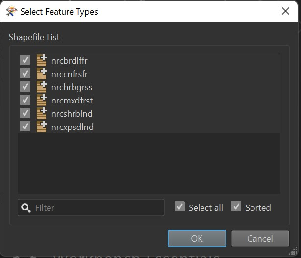
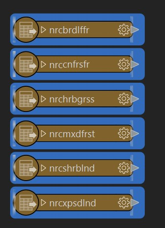
- Drag and Drop the 6 shapefiles found in L:\GEOG413\lab04\vegitation onto the workspace
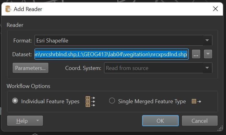
A popup will appear to Add Reader, it should detect the format as Esri Shapefile and we will allow it to read the coordinate system from the source. - Add the pop_places shapefile from L:\GEOG413\lab04
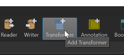
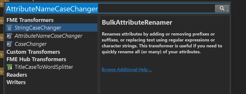
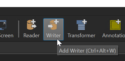
The next issue to address is that the shapefiles use capital letters extensively, in a perfect world it is easier in PSQL to avoid capital letters in attribute names. Along the top menu bar find the Add Transformer option
Set the Format to PostGIS, then under Connection add a database connection, use the credentials for your personal database. Under Table Definition select ‘Dynamic’
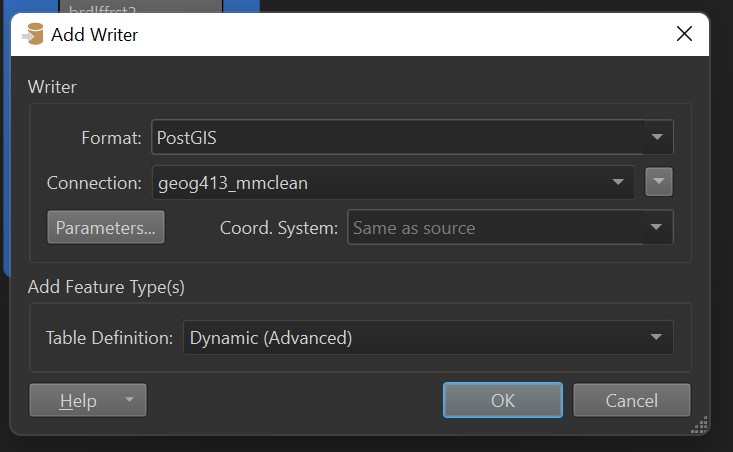
Now press the gear on the new writer to change its settings, and set the table qualifier to lab4 (this will create a new schema called lab4.
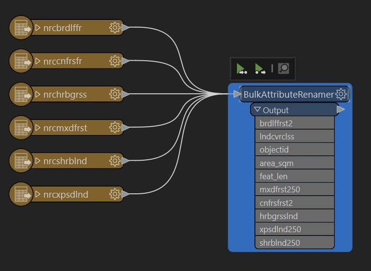
The final graph should look similar to this
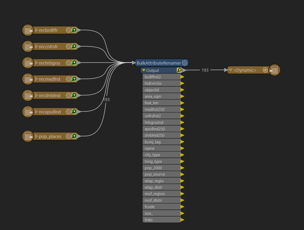
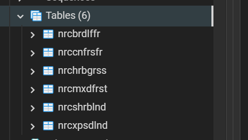
This process will take time, it is adding several million polygons to the database. While it runs in the background feel free to open pgAdmin and check to see the tables are being added to your database.
Spatial Data Types
Before proceeding let us take a minute to talk about the datatypes used by PostGIS, the keen-eyed among you may have noticed that FME added the features with a Geometry column, however, geography could have also been an option. Which one you choose will depend on the data, the general rule of thumb is that Geometry is faster but runs within projected coordinate systems; Geography while a slower computation time represents points on a datum and will account for the curvature of the earth, especially important when measuring long distances if high precision is needed.
What does this mean for us? All of the data used was added with the BC Albers SRID into geometry, in this case, all measurements by default will come back in meters as this is the unit specified in BC Albers. Additionally, all distances are calculated using Cartesian Coordinates which is relatively fast.
The Geography type is useful for latitude and longitude, as returning measurements of unprojected data ESPG:4326 in the geometry type would be returned in the default units, in this case, degrees, how long is a degree?
Tips for success:
- For small geographic areas (up to a province) you likely want to use projected data with geometry types. For larger areas consider using the Geography type.
- Always be aware of the projections used in tables, and avoid having multiple projections in a single database, if you must always remember to transform to a common system inside of queries. This can be especially dangerous if crossing UTM zones!
Spatial Queries
In pgAdmin open the Query Tool, for the first query start with the simple
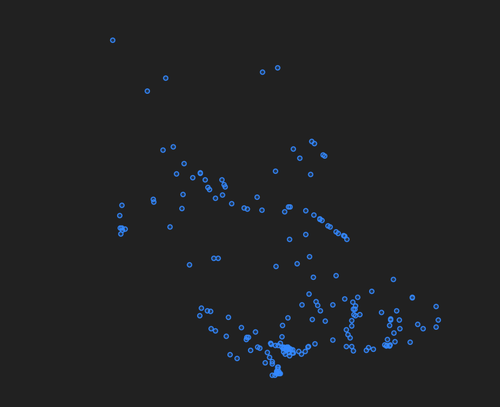
SELECT * FROM lab4.pop_places;
The results returned will look just like the attribute table from desktop GIS software, with the addition of the geom column, you will also notice a map logo by this column, simply click on this to see a preview of the data.

Projections
As mentioned before inside of PostGIS you need to make sure to stay on top of your projections as data is returned based upon the projection it was saved in. In the database the projections used are identified by a records SRID (Spatial Reference ID), these SRIDs were standardized by the European Petroleum Survey Group, and thus may be referenced as EPSG codes. You can look up projections on this website https://spatialreference.org/ref/epsg/. For example
If we want to see the coordinates of the places above additional columns can be added to the query results.
SELECT ST_X(geom), ST_Y(geom), ST_SRID(geom), * FROM lab4.pop_places;
The coordinates returned are in BC Albers, if you want points you could use them in your GPS you may want decimal degrees, this can be done using ST_TRANSFORM, for example
SELECT ST_X(ST_TRANSFORM(geom, 4326)), ST_Y(ST_TRANSFORM(geom, 4326)), ST_SRID(ST_TRANSFORM(geom, 4326)), * FROM lab4.pop_places;
Note: You will also find a function called ST_SETSRID() this function changes the SRID of geometry without changing the coordinates, this function is useful if the SRID code is missing for some reason, however, can lead to invalid data.
UTM can be a particularly challenging coordinate system in PostGIS as the zone is encoded in the SRID, thus measuring distances between features across the zones may yield unexpected results. What are some options to overcome this?
Topological Functions
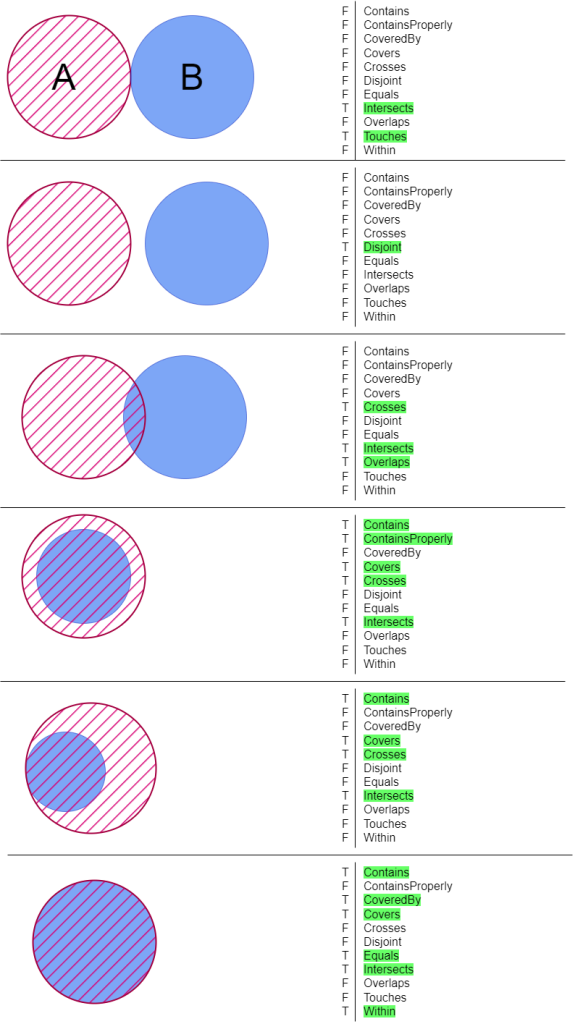
Before performing spatial joins it is essential to first understand the Topological Functions available. When determining what function to use it is very helpful to reference the available documentation from PostGIS https://postgis.net/docs/reference.html#idm12212, each function has a very precise meaning. For example at first glance intersect and touches may sound similar but there is a difference. intersect is true if two geometries have any point in common, where as touches requires that a border touches.
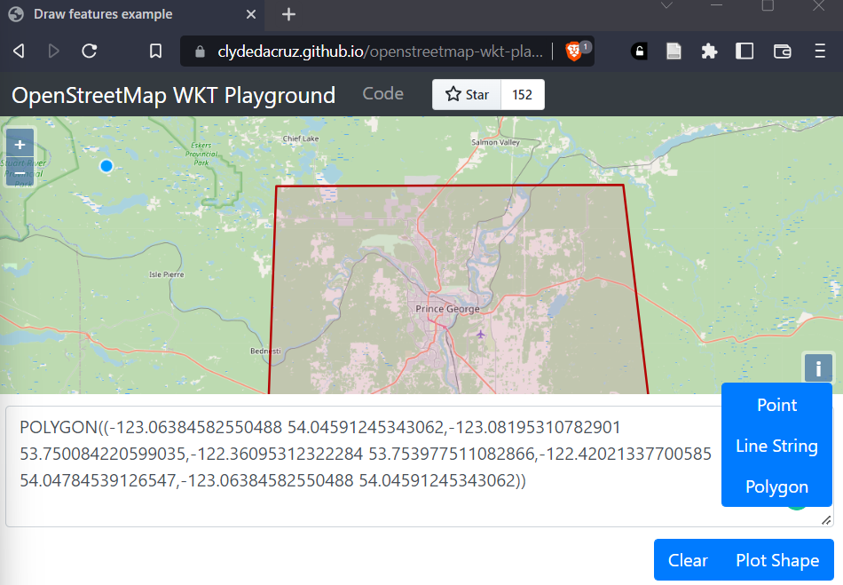
For our first spatial selections, we will make use of Well Known Text geometries generated from this webpage https://clydedacruz.github.io/openstreetmap-wkt-playground/ when the page loads press clear then draw a polygon coving a small portion of BC, perhaps a city and it’s surroundings.
nrcbrdlffr -> Broadleaf Forest
nrccnfrsfr -> Coniferous Forest
nrchrbgrss -> Grassland
nrcmxdfrst -> Mixed Forest
nrshrblnd -> Shurbland
nrcxpsdlnd -> Exposed Land
If you wanted to select all the bare land within your polygon you will have a query like below. One of the biggest lessons to take at this point is to keep your code organized; technically this could be only 2 lines of code however that would be extremely hard to read. While SQL does not place any meaning on indentation, humans trying to understand what is happening do. The exact way in which you format your code is not as important as being consistent; when working on teams this often means working with your teams preference over your own so the entire codebase can remain consistent.
SELECT * FROM lab4.nrcshrblnd
WHERE ST_Intersects(geom,
					ST_Transform(
						ST_GeomFromText('POLYGON((-123.06384582550488 54.04591245343062,
										-123.08195310782901 53.750084220599035,
										-122.36095312322284 53.753977511082866,
										-122.42021337700585 54.04784539126547,
										-123.06384582550488 54.04591245343062))',4326),
					3005))
This is also a good opportunity to bring up the importance of comments, the above code is still hard to understand one way to make it better would be adding comments.
SELECT * FROM lab4.nrcshrblnd --Bareland vegitation layer
WHERE ST_Intersects(geom,
					ST_Transform(
						--WKT geometry is bounding box coving Prince George BC
						ST_GeomFromText('POLYGON((-123.06384582550488 54.04591245343062,
										-123.08195310782901 53.750084220599035,
										-122.36095312322284 53.753977511082866,
										-122.42021337700585 54.04784539126547,
										-123.06384582550488 54.04591245343062))',4326), --WKT is SRID 4326
					3005)) --Transform to BC Albers, match vegitation layer
It doesn’t take a lot of comments to provide helpful context to your queries, especially important when dealing with SRID codes.
Take some time here, try some of the different Topological functions, or put the custom geometry first.
Spatial Joins
Joining based on location is one of the fundamental GIS database options, as often in analysis the relationship between records is their location as opposed to a text-based attribute. Given the question of determining what percentage of land surrounding each city in BC (for 5km from the city center) is grassland; what information must we have to answer this question?
- What is the area surrounding each city?
- What inside of that area is grassland?
- How does this area compare to the area of the buffer?
A logical first step will be to apply a buffer to get the area for the cities; using the database this can be done on the fly without making a new layer.
SELECT name, ST_Buffer(geom,5000) AS city_area FROM lab4.pop_places;
At this stage, we have the cities with an area, which can now be joined to the grassland layer. First, start by building out the query to make this a sub-query named city
SELECT * FROM (SELECT name, ST_Buffer(geom,5000) AS city_area FROM lab4.pop_places) city;
This query does not perform any differently, however, gives us a way to identify the new buffers (city.geom).
SELECT * FROM (SELECT name, ST_Buffer(geom,5000) AS city_area FROM lab4.pop_places) city
JOIN lab4.nrchrbgrss ON ST_Intersects(city.city_area, nrchrbgrss.geom)
This can then be built out further by calculating area using aggregate functions and the GROUP BY clause
SELECT city.name, MAX(ST_Area(city.city_area)) AS city_area, SUM(nrchrbgrss.area_sqm) AS grassland
FROM (SELECT name, ST_Buffer(geom,5000) AS city_area FROM lab4.pop_places) city
JOIN lab4.nrchrbgrss ON ST_Intersects(city.city_area, nrchrbgrss.geom)
GROUP BY city.name
There is however a problem with this query, can anybody see what the issue is? What are your ideas for fixing it?
Solution
ST_Intersects finds all of the polygons that have an intersection, however, this does not actually cut the boundaries, to do this we must use the ST_Intersection() function.
SELECT city.name, MAX(ST_Area(city.city_area)) AS city_area, SUM(ST_AREA(ST_Intersection(nrchrbgrss.geom, city.city_area))) AS grassland
FROM (SELECT name, ST_Buffer(geom,5000) AS city_area FROM lab4.pop_places) city
JOIN lab4.nrchrbgrss ON ST_Intersects(city.city_area, nrchrbgrss.geom)
GROUP BY city.name;
Finally, the percentage must be calculated. This can be done by modifying the first line, however, I find it a little bit cleaner to insert this all into a new subquery to make a shorter SELECT statement for readability, and add an ORDER BY to sort the data to show cities with the highest coverage first.
SELECT name, ROUND((grassland/city_area*100)::numeric, 2) AS cover_pct, city_area, grassland, geom
FROM
    (SELECT city.name,
    ROUND(MAX(ST_Area(city.city_area))) AS city_area,
    ROUND(SUM(ST_AREA(ST_Intersection(nrchrbgrss.geom, city.city_area)))) AS grassland,
    ST_Intersection(nrchrbgrss.geom, city.city_area) AS geom
    FROM
        (SELECT name, ST_Buffer(geom, 5000) AS city_area
        FROM lab4.pop_places) city
        JOIN lab4.nrchrbgrss ON ST_Intersects(city.city_area, nrchrbgrss.geom)
        GROUP BY city.name
    ) cities_grassland
ORDER BY grassland DESC
These queries are still relatively small some quick tips before we move on, first is query structure when in doubt you can always start with a skeleton of
SELECT
FROM
JOIN
WHERE
GROUP BY
ORDER BY
Removing any of the sections that are not needed.
When writing queries do not try to make the entire query in one go, start with simple queries, and combining into more complex questions.
At this stage, you should also be starting to notice the power of SQL, while it is true that you likely could have answered this question faster with desktop GIS. What about when the question changes, what if a client wants to change the radius from the city? What if more cities are added to the map? How will your results change as vegetation maps are updated?
Spatial Indexes
Another important component of spatial databases is indexing, most commonly in PostGIS, this will be the GIST index. http://postgis.net/workshops/postgis-intro/indexing.html Indexes are very easy to create, so easy infact that FME created indexes for us after inserting the data, if you expand the table in pgAdmin you will be able to see it.
CREATE INDEX <table>_geom_idx
  ON <table>
  USING GIST (geom);
It is also worth noting that over time an index may become stale, if your database starts to slow after changing many records it may need to be reindexed.
If you want to know how big an impact these indexes have, run the grassland query noting how long it takes to run (should be about 6 seconds). If you change (please do not actually run this) the join from ST_Intersects() to _ST_Intersects it will ignore the indexes, in this case, the query will ignore the index, and runtime will be extended to about 30 minutes!
Viewing Your Data
To view this data in QGIS we can enter the query directly, but first, we need to put the geometry column back. Note that when using group by every column must have an aggregate applied, in this case, we will use ST_Union().
SELECT name, ROUND((grassland/city_area*100)::numeric, 2) AS cover_pct, city_area, grassland, geom
FROM
    (SELECT city.name,
    ROUND(MAX(ST_Area(city.city_area))) AS city_area,
    ROUND(SUM(ST_AREA(ST_Intersection(nrchrbgrss.geom, city.city_area)))) AS grassland,
	ST_Union(ST_Intersection(nrchrbgrss.geom, city.city_area)) AS geom
    FROM
        (SELECT name, ST_Buffer(geom, 5000) AS city_area
        FROM lab4.pop_places) city
        JOIN lab4.nrchrbgrss ON ST_Intersects(city.city_area, nrchrbgrss.geom)
        GROUP BY city.name
    ) cities_grassland
ORDER BY grassland DESC
In QGIS right click on your database, and choose Execute SQL, you can then paste and execute this query, after it completes along the bottom an option to add a layer will appear, set the Geometry column, and press Load Layer.
Next, we will use a feature of Postgresql known as Views to simplify this process, you can think of a view as naming a select query for easy reference, they also provide the advantage if the view is changed any software referencing the view will also receive the updates.
In pgAdmin add the create view command directly before the query, and run; it should output CREATE VIEW Query returned successfully as opposed to data results.
CREATE VIEW lab4.city_grassland AS
return to QGIS, right-click on your database, and refresh, you will notice that your view is now available as a layer.
The next issue arising however is that calculating the intersection every time data is viewed is a slow process, for databases that rarely have changes in data a materialized view allows for these calculations to be done beforehand. Thes are created like so
CREATE MATERIALIZED VIEW lab4.city_grassland_material AS
However, data is a materialized view will go stale, if data is changed the view must be recalculated with the command
REFRESH MATERIALIZED VIEW lab4.city_grassland_material
Try turning off the previously added layers and using just the materialized view, how does this affect performance?
Out of the scope of this course, something you should be aware that exists is scheduled actions (ie. recalculate a materialized view every night); and triggers, common use of triggers would be to say when data is inserted into table x, refresh materialized view y.
Assignment
As practice is essential for masting this material today’s assignment is broken into two parts first is group work; for this section, you must submit answers, but are encouraged to talk with classmates or your instructor to work towards a solution, and should be completed before leaving the lab. The remainder of the assignment will be a personal assignment, you may ask your instructor for clarification, but all work should be your own.
Please submit all code as selectable text, you may either paste it into your word document or save it as .sql files and include it with the submission, please no screenshots of the code!
Group Assignment (1 mark)
Using the data loaded for this lab, a biologist comes to you with a question they want to identify all the grassland on Vancouver Island that is within 500m of conifer forest, and also at least 25km from any populated places. Develop a query to produce this result, and display results in QGIS.
You can take Vancouver Island to be defined by this WKT
'POLYGON((-124.16919708251953 49.26018706362072,
-124.10327911376953 49.07386590128539,
-123.78879547119139 49.10983779052441,
-123.90209197998047 49.27542086174671,
-124.16919708251953 49.26018706362072))'
- What are the high-level steps needed to complete this task? You should have at least 3 main components
- For each component identified what describe SQL commands you need
- Put all the pieces together into one query to answer the question
- Create a materialized view and display in QGIS, and submit a screenshot of the display.
Personal Assignment (4 marks)
Add the data in the census folder of the lab to your database, two tables one with da_pop_all_of_bc, and another with the census boundaries lda_000a16a_e.
In your database write queries to join these tables and answer the following questions.
What is the total population for each Census Division (CDUID)?
What is the total area for each Election Region (ERUID)?
What is the population density for each Census Sub Division (CSDUID)?