In todays lab we will be working with Enterprise Database Management Systems (DBMS). First looking at conceptual design, then logical design, and finishing with with SQL or Structured Query Language. While we will not be working with spatial data today, this weeks lab forms an important foundation for next weeks lab section.
Why use a database?
Before we start building databases lets take a quick look at why we may want to use one, the why’s generally come down to one of the following points.
- Sharing Data – A database can be connected to by many people at one time, especially in the case of editing, where a shapefile would be edited by only a single individual.
- Security – Databases provide the ability to grant different users to different data, as well as revoke access should needs change.
- Single source of truth – In an organization connecting to a database means that as data is changed processes that depend upon this information can also be updated. A simple example of this would be a customer updating their address and various departments needing this information. For a geospatial example if our maps pull data from a database that means that maps can always be re-created with newest possible data.
- Performance – Database systems can provide very high performance access to very large datasets; especially when designed by a skilled Database Administrator (DBA). Database may be used to relate files that would be too large to efficiently share as files, tuning indexes, and physical data layout can also lead to improvements.
- Integration of Systems – An example of a task that you may be asked to perform as a GIS professional may be to produce a map of customers for example. In this example a company may have an existing Inventory Management System (IMS) or Customer Relationship Management System (CRM) containing information about customers including addresses. Our GIS software will not open these databases by default, however mastering DB access will allow you to select data from the database, apply geocoding to addresses and then make maps or apply spatial analysis to datasets that did not start in a GIS.
Connecting to our first database
We will start todays lab by looking at the TRIM roads layer accessed from both a shapefile and a PostGIS database.
Start by opening QGIS and adding the shapefile found in L:\GEOG413\lab03\trim\trim_roads.shp you will notice this file is taking a very long time to load. While its loading you will see the Browser Panel along the left of QGIS has various options one of them is PostgreSQL (icon is an elephant), right click on this and pick “New Connection” and fill out the form with below information
- Name: TRIMv1
- Host: pgadmin.gis.unbc.ca
- Port: 5432
- Database: trim
- Authentication: Select the ‘Basic Tab’
Username: sde
Password: unbc-user
Store: checked - Test configuration (if successful press save).
It may take the Browser a while to index the database tables, a faster option is to go to the Database option along the top menu, open DB Manager, expand PostGIS -> TRIMv1 -> trim, and find the layer road__trim and double click it to add to the map.
After you have a chance to zoom around and see how the layers perform, right click on them in the Layers pane and remove to give the computer a bit of a break.
Saving data to the database
Next we will save some data into a database, you had read only permission to the trim DB however for this course you have also been given a DB with full access we will put some data into here. We will use a layer of a bit more manageable size the airports from TRIM, you can add this to QGIS from the following location L:\GEOG413\lab03\trim\trim_airfield.shp
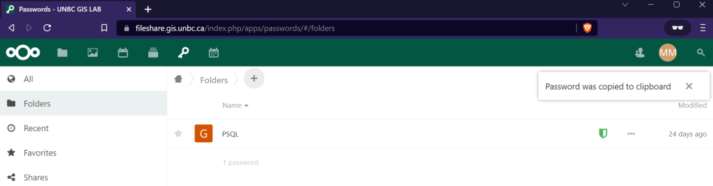
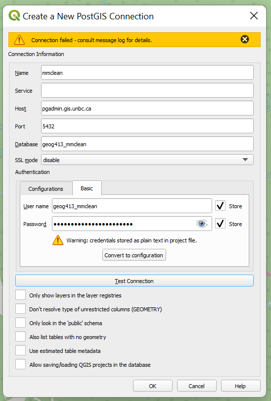
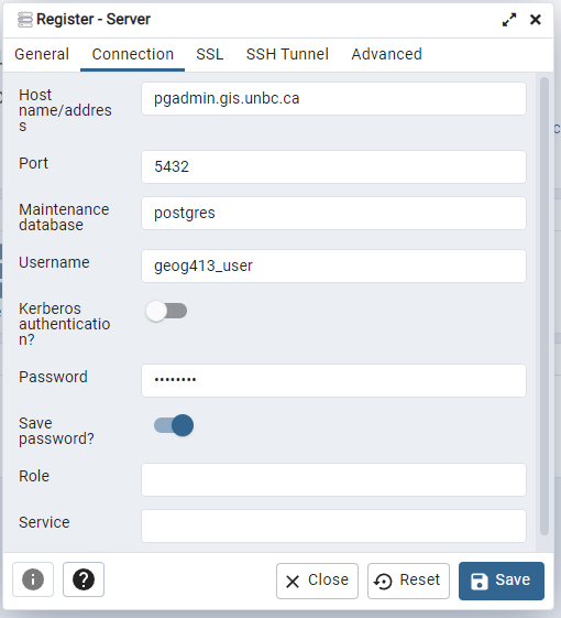
When connecting to the database your database and user will be of the same format, geog413_<username> for example my database is geog413_mmclean, and user is geog413_mmclean. You can get your password from https://fileshare.gis.unbc.ca click on the key in the top menu, in the password manager you will see a secret named psql, simply click on it and your unique password will be copied to the clipboard.
Now just as we connected to the trim database in QGIS do the same but with the database unique to your user.
To add the layer open DB Manager as before and select the database you just added, and press the “ImportLayer/File” button, here we have the following options
- Input – This is any layer you have open in QGIS and will be what we save to the database.
- Schema – We will talk more about these below for now just leave as public
- Table – What will this layer be called in the database
- Primary Key – Databases should almost always have a primary key to ensure records are uniqe
- Geometry Column – This is the column that the actual shape is saved to, convention says this is named ‘geom’ while this can be changed most software defaults to looking for this column.
- Source SRID – Helps to make sure QGIS understands what layer was input, important if the file loaded as an unknow CRS.
- Target SRID – What type of geometry do you want stored in your database? Convention would say you generally want to be consistent within the database, for now we will just use the default of BC Albers (EPSG:3005), however it is very common to also see EPSG 4326 (unprojected lat/lon), or 3857 (Pseudo Web Mercator) if the project does not have specific requirements). Not all libraries will read this information by default so mixing your SRID can cause headaches later.
- Convert to lowercase – Again this is a convention when writing PostgreSQL any occurrences of capitol letters will need to be surrounded by quotes as such it is often simpler to ensure that all columns do not contain any capitols.
- Create Spatial Index – This will create an index that allows the database to search for geometry in specified extents without needed to calculation the position of every point later on, this results in substantially faster queries especially when selecting only a subset of the data contained.
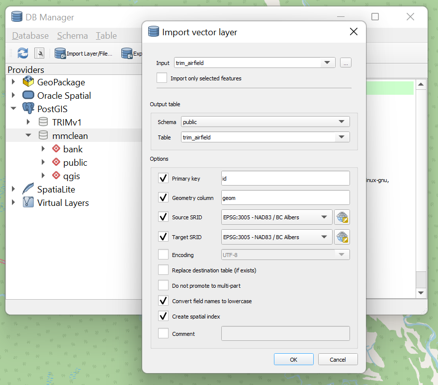
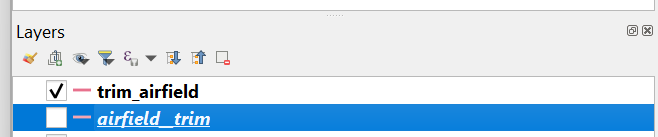
Press OK and the layer will be added to the database (by default it will be added turned off immediately below the original source data).
At this level it is easy to think of a database server much like a file server; however this is Advanced GIS so we will be taking a look into how to not just place data into a database but how to design the structures that will store data.
How is a database structured?
When looking at a database we have a hierarchy used to organize data with the following primary elements.
Database Server: At the highest level this is a single server that will store all of our database, a company may have one or may have many. For an analogy of considering a database files on your computer the Database Server is your computer. For this course this server is pgadmin.gis.unbc.ca.
Database: A database is the highest level of organization, typically we would want all the data connected to a specific project (or at least the data we will be editing) to be within a single database. For the computer analogy think of this as a hard drive. For this course it will be geog413_username.
Schema: Schemas are logical sections within a database, and typically queries are done within an individual schema, though no always. Schemas help to provide logical and physical structure to our databases. Logically they provide organization and allow setting permissions to the schema per user or group. Physically (outside the scope of this course) they can also provide separation for physical storage, you might put heavily used data on SSD’s while less frequently accessed data is stored on more economical HDD’s. Think of this as folders on your hard drive (though in this case subfolders are not possible).
Tables: Tables are where data is actually stored, and function similar to a spreadsheet. Tables are defined as a set of columns with specified content along with data type, and if it is mandatory the column be used, or matches specific formats.
Records: This is the data in the database, and are something along the lines of a row in a spreadsheet.
Conceptual Design of Databases
When working with DMBS we are specifically looking at relational databases; at a high level this means that we will have a series of ‘entities’ that can be linked using ‘relations’.
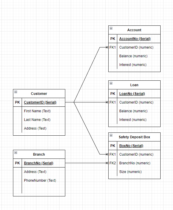
An Entity can be thought of as the minimal representation of an object, and its attributes. A subset of these attributes can be used to define unique instances of this Entity. As an example lets say we want to store some banking information in a database; a person could have debts, loans or safety deposit boxes, and those boxes will be in a physical branch. We will model this using an Entity Relationship Diagram (ER Diagram).
Go to https://fileshare.gis.unbc.ca, in the upper left corner of the main pane there is a ‘+’ use this to create a folder for GEOG413, and then inside a folder for Lab3. Once inside this folder press + again and pick new diagram, give it a name and press the arrow to start.
When the diagram loads choose Blank Diagram and Create. Along the left pane expand Entity Relation, this will have all of the shapes we need for todays lab. ER is a very expressive way of showing databases, for the purposes of this class we will only be looking at the very basics at the conceptual level using only Rectangles for Entities, and Rhombus for Relationships connected by lines (If you are interested in the more complete representation of symbols Lucidchart has a great resource https://www.lucidchart.com/pages/er-diagrams).
Lets all make a chart like the one below:
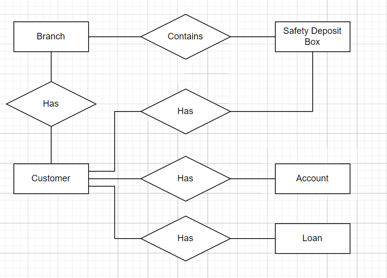
In general we want Entities to be as small as possible to avoid repeating data wherever possible.
Logical Design of a Database
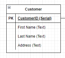
With our conceptual model of the database complete, now it becomes time to start thinking about how this data will be stored into tables. To do this we will translate each entity into a table, and the relationships will be represented with keys. In databases there are 2 types of keys; Primary Keys are the column or set of columns in the table that can uniquely identify each record in the table. Foreign Keys are the column or set of columns that can be used to look up records in another table, often matching that tables primary key.
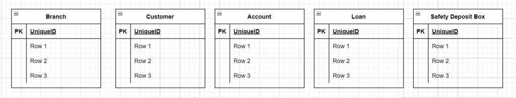
In your diagram start by adding the entities by adding and naming 5 of the table objects, it should look like below.
The next step will be to determine what attributes each entity needs, and specifically the PK, lets say that gives you something such as this.
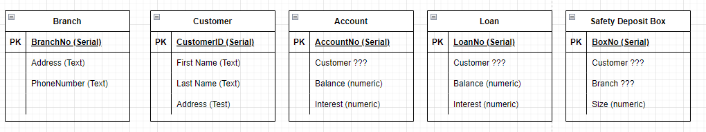
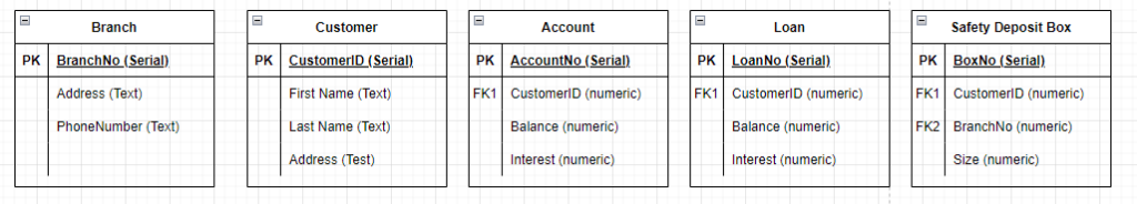
At this stage we now that Account, Loan, and Safety Deposit Box need to relate to the customer, this is done by identifying the Foreign Key (again typically the PK.
SQL
Once we have a conceptual idea of what our data should look like, we can turn our attention to implementing with computer code.
For security reasons each of you has already been provided with a database, normally the first stage of SQL programming would to complete this step, for reference this is the code that produced the database you will be using.
CREATE DATABASE "geog413_username"
    WITH
    OWNER = geog413_username
    ENCODING = 'UTF8'
    CONNECTION LIMIT = -1
    IS_TEMPLATE = False;
In the above code only the first line is strictly needed, however we say WITH to tell the server we will provide additional information, grant the owner of the database, specify how text is stored, and set the connection limit (-1 is unlimited), and we are not using a template. All SQL ‘Queries’ are finished with a “;”.
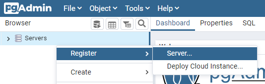
To access your database go to https://pgadmin.gis.unbc.ca/ and login with your standard UNBC credentials. This is pgAdmin 4 and is not actually the database, just a piece of software we use to administer databases. To connect to the server right click on server in the upper left corner, choose register, and Server.
Give the connection a friendly name
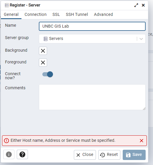
Press save and you should now be able to see your personal database in the side bar.
Select your database nd open the query tool from the top menu bar.
When working with databases there are four basic operations Create, Read, Update, Delete often referred to as CRUD.
- Create – We use the CREATE keyword to make new databases, schemas and tables. At the record level creation will be done via the INSERT command.
- Read – After we have data in our database, it can be read via the SELECT command.
- Update – Changing records already in a table are updated as opposed to inserted.
- Delete – This is most commonly achieved via the DROP command.
We will go through the basics of these commands below.
CREATE
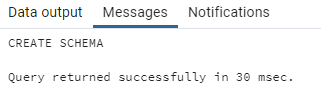
First we will create a new schema to hold the tables for the above example, in our database. This is very easy to to simply enter the command
CREATE SCHEMA bank;
Press the play button and you should see the following output
CREATE TABLE bank.customer
(
    customerid serial NOT NULL,
    first_name text,
    last_name text,
  	address text,
    CONSTRAINT customer_pkey PRIMARY KEY (customerid)
);- First we are creating the table customer inside the schema bank, by default tables will go into the public schema. That is to say “CREATE TABLE customer” is the same as “CREATE TABLE public.customer”
- All of the columns are in brackets
- Each column has a name, data type and optionally modifiers. For the case of customerid the type is serial (integer where value increases by 1 every time a record is inserted), and we set it to NOT NULL that is every record in branch must have a branch number.
- The address column holds text. How would we change this if we wanted to enforce that every branch has an address?
- Same for phone.
- Finally we can add constraints, in this case defining the primary key is customerid, this constraint implies that customerid is not null, and is unique.
Next to see how the Foreign Key works we will create the account table, again referencing the ER diagram.
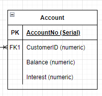
CREATE TABLE bank.account
(
    accountno serial NOT NULL,
	customerid integer,
    balance numeric,
  	interest numeric,
    CONSTRAINT account_pkey PRIMARY KEY (accountno),
	CONSTRAINT customer_fkey FOREIGN KEY (customerid) REFERENCES bank.customer(customerid)
);
The complete code to build this is below. (If you have errors in your schema from before you can simply right click in pgAdmin and Drop it; note that this is a permanent and irreversible deletion)
CREATE SCHEMA IF NOT EXISTS bank;

CREATE TABLE IF NOT EXISTS bank.customer
(
    customerid serial NOT NULL,
    first_name text,
    last_name text,
  	address text,
    CONSTRAINT customer_pkey PRIMARY KEY (customerid)
);

CREATE TABLE IF NOT EXISTS bank.account
(
    accountno serial NOT NULL,
	customerid integer,
    balance numeric,
  	interest numeric,
    CONSTRAINT account_pkey PRIMARY KEY (accountno),
	CONSTRAINT customer_fkey FOREIGN KEY (customerid) REFERENCES bank.customer(customerid)
);

CREATE TABLE IF NOT EXISTS bank.branch
(
    branchno serial NOT NULL,
  	address text,
	phone text,
    CONSTRAINT branch_pkey PRIMARY KEY (branchno)
);

CREATE TABLE IF NOT EXISTS bank.loan
(
    loanno serial NOT NULL,
	customerid integer,
    balance numeric,
  	interest numeric,
    CONSTRAINT loan_pkey PRIMARY KEY (loanno),
	CONSTRAINT customer_fkey FOREIGN KEY (customerid) REFERENCES bank.customer(customerid)
);

CREATE TABLE IF NOT EXISTS bank.depositbox
(
    boxno serial NOT NULL,
	customerid integer,
    branchno integer,
  	size integer,
    CONSTRAINT box_pkey PRIMARY KEY (boxno),
	CONSTRAINT customer_fkey FOREIGN KEY (customerid) REFERENCES bank.customer(customerid),
	CONSTRAINT branch_fkey FOREIGN KEY (branchno) REFERENCES bank.branch(branchno)
);
INSERT
Now that the schema for this simplified DB example, it is time to start adding data, this is done through the INSERT statement. Lets add John Doe to our database of customers (note the customer ID is 100, this will be important later).
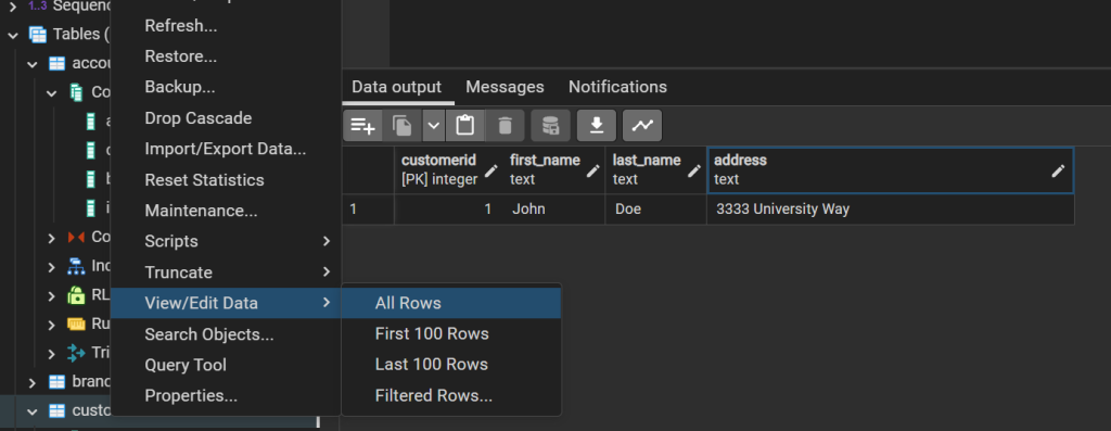
INSERT INTO bank.customer VALUES (100, 'John', 'Doe', '3333 University Way');
In this case values were provided as a list in the order the column’s appeared when creating the schema. You can confirm the data is present by expanding the Tables inside of bank, and right click on customer and choose view data.
However while this is convenient it means than any changes to the schema may break this in the future if the order of columns change. An option to make the code more robust would be to specify the columns we want to fill.
INSERT INTO bank.customer (last_name, first_name, address) VALUES ('Doe', 'Jane', '3333 University Way');In this case we defined the order the data would be passed, and also what data would be passed. Notice in this example the customerid was omitted, this is because the data type serial has a default value, and this default will increase with every use. Had we inserted John Doe as customer 1, serial would have tried to start at 1, breaking the primary key constraint; generally you should avoid ever manually setting serial keys, as in this example this will break for the 100th customer.
SELECT
Previously when viewing data, pgAdmin auto filled a query that looked something like the following
SELECT * FROM bank.customer
ORDER BY customerid ASC;
This query says that we wish to see all the columns (*) from bank.customer, and to display them in a sorted list. If you go back to a normal query window (you cannot edit the auto generated queries) this can be modified to provide only specific information the most common way of filtering results would be the WHERE clause. For example
SELECT * FROM bank.customer
WHERE first_name = 'John' AND last_name = 'Doe'
ORDER BY customerid ASC
And if you only wanted speific information you might replace the * with column names, like so
SELECT customerid FROM bank.customer
WHERE first_name = 'John' AND last_name = 'Doe'
ORDER BY customerid ASC
Nested Queries
So far data has only been added to the customer table, adding an account for example has the extra detail of a Foreign Key, a record with a Foreign Key cannot be added unless that key already exists as the primary key of the referenced table. Try the below query to add an account for customer 25, with a $0 balance and 0.5% interest rate and see what happens
INSERT INTO bank.account (customerid, balance, interest) VALUES (25, 0, .5);
In this case there is no customer 25 so it fails; to create this account for John Doe their customerno must be known; or the database can be asked for it, by replacing a value with a query surrounded by brackets.
INSERT INTO bank.account (customerid, balance, interest) VALUES (
	(SELECT customerid FROM bank.customer
	WHERE first_name = 'John' AND last_name = 'Doe'
	ORDER BY customerid ASC),
0, .05);
If you view the data in the account table there should now be an account belonging to customerid 100. The purpose of nesting is that it allows complex queries to be built of simple parts; in the real world a query may contain 10’s or even a hundred plus lines of SQL but that does not mean they need to be written a a single piece they can be slowly built up.
Joins
Before proceeding it will be useful to have some more data in the database, the below query will remove any records created to date reset the serial id’s, and then insert data into the tables.
--Remove data already in database, CASCADE will remove data in tables with Forign Key Restraints
TRUNCATE bank.customer, bank.branch CASCADE;
--Reset all SEQUENCES to 0, insert statments below are using explicit id's
ALTER SEQUENCE bank.account_accountno_seq RESTART WITH 1;
ALTER SEQUENCE bank.branch_branchno_seq RESTART WITH 1;
ALTER SEQUENCE bank.customer_customerid_seq RESTART WITH 1;
ALTER SEQUENCE bank.depositbox_boxno_seq RESTART WITH 1;
ALTER SEQUENCE bank.loan_loanno_seq RESTART WITH 1;

--Add Data to branch table
INSERT INTO bank.branch (address, phone) VALUES ('First Ave, Mytown', '555-1234');
INSERT INTO bank.branch (address, phone) VALUES ('Castle St, Kingdom', '555-5474');
INSERT INTO bank.branch (address, phone) VALUES ('Motocar Way, Racetown', '555-4444');

--Add Data to customer table
INSERT INTO bank.customer (last_name, first_name, address) VALUES ('Doe', 'John', '3333 University Way');
INSERT INTO bank.customer (last_name, first_name, address) VALUES ('Doe', 'Jane', '3333 University Way');
INSERT INTO bank.customer (last_name, first_name, address) VALUES ('Smith', 'Luke', 'Someplace Prince George, BC');
INSERT INTO bank.customer (last_name, first_name, address) VALUES ('Myth', 'Buster', 'San Francisco, California');
INSERT INTO bank.customer (last_name, first_name, address) VALUES ('Lovelace', 'Adda', 'Nottingham, England');

--Add Data to account table
INSERT INTO bank.account (customerid, balance, interest) VALUES (1, 3000, 0.4);
INSERT INTO bank.account (customerid, balance, interest) VALUES (1, 8900, 0.4);
INSERT INTO bank.account (customerid, balance, interest) VALUES (2, 350000, 0.5);
INSERT INTO bank.account (customerid, balance, interest) VALUES (2, 88000, 0.2);
INSERT INTO bank.account (customerid, balance, interest) VALUES (2, 200, 0.4);
INSERT INTO bank.account (customerid, balance, interest) VALUES (3, 40, 0.3);
INSERT INTO bank.account (customerid, balance, interest) VALUES (4, 8745, 0.4);
INSERT INTO bank.account (customerid, balance, interest) VALUES (4, 300, 0.5);
INSERT INTO bank.account (customerid, balance, interest) VALUES (5, 175, 0.5);
INSERT INTO bank.account (customerid, balance, interest) VALUES (5, 25466, 0.4);
INSERT INTO bank.account (customerid, balance, interest) VALUES (5, 500000, 0.2);
INSERT INTO bank.account (customerid, balance, interest) VALUES (5, 20400, 0.3);

--Add Data to loan table
INSERT INTO bank.loan (customerid, balance, interest) VALUES (1, 65458, 3.4);
INSERT INTO bank.loan (customerid, balance, interest) VALUES (1, 45464, 2.4);
INSERT INTO bank.loan (customerid, balance, interest) VALUES (2, 545656, 1.5);
INSERT INTO bank.loan (customerid, balance, interest) VALUES (2, 445454, 2.2);
INSERT INTO bank.loan (customerid, balance, interest) VALUES (2, 1447, 3.4);
INSERT INTO bank.loan (customerid, balance, interest) VALUES (3, 4000, 4.3);
INSERT INTO bank.loan (customerid, balance, interest) VALUES (3, 8444, 1.4);
INSERT INTO bank.loan (customerid, balance, interest) VALUES (4, 344, 5.5);
INSERT INTO bank.loan (customerid, balance, interest) VALUES (5, 144475, 4.5);
INSERT INTO bank.loan (customerid, balance, interest) VALUES (5, 25556, 3.4);
INSERT INTO bank.loan (customerid, balance, interest) VALUES (5, 50400, 4.2);
INSERT INTO bank.loan (customerid, balance, interest) VALUES (5, 240, 3.3);

--Add Data to depositbox table
INSERT INTO bank.depositbox(customerid, branchno, size) VALUES (1, 1, 1);
INSERT INTO bank.depositbox(customerid, branchno, size) VALUES (2, 1, 2);
INSERT INTO bank.depositbox(customerid, branchno, size) VALUES (3, 1, 3);
INSERT INTO bank.depositbox(customerid, branchno, size) VALUES (4, 2, 2);
INSERT INTO bank.depositbox(customerid, branchno, size) VALUES (5, 3, 1);
With data in the database the it starts to become more obvious why is is called a relational database when we go to ask a question, for example what is the bank balance of John Doe? To answer this we need to use the JOIN command as seen below.
SELECT * FROM bank.customer
JOIN bank.account ON account.customerid = customer.customerid;
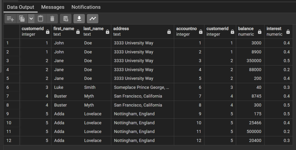
This result gives one row per customer per account. By default this is giving an inner join, that is the record must appear in both tables, in this case because of the Foreign Key restraints all accounts must have a customer, but the same is not true in reverse. What time of join might we use to ensure that all customers are present in this list?
Additionally we may want to know how much each customer has in loans as well, at this point it may be tempting to simply add another join like so
SELECT * FROM bank.customer
LEFT JOIN bank.account ON account.customerid = customer.customerid
JOIN bank.loan ON loan.customerid = customer.customerid;
However the problem here is that the first join left multiple customer ID’s for each customer, there was 12 accounts, and 12 loans so we expect to get 24 rows back, but what came back was 33 rows. There are a couple of options to solve this the less elegant solution would be to UNION joins, in this case adding a column past the wild card to indicate weather the balance is positive or negitive.
SELECT *, 'credit' as acct_type FROM bank.customer
JOIN bank.account ON account.customerid = customer.customerid

UNION

SELECT *, 'debt' as acct_type FROM bank.customer
JOIN bank.loan ON loan.customerid = customer.customerid;
another option would be to make it so there was only one entry per customer id.
Aggregation
Aggregate functions are one of the most basic forms of analysis that can be done in a database and are used to reduce many rows down to few by combining them, providing an aggregate value. While we are currently working with standard databases the keen among you may already be considering how such functions might be used to get average population, or number of people located within a region. In the above example we got a list of all accounts, but what if we just wanted to know how much money each customer had? We could do that using aggregation for example.
SELECT customer.customerid, first_name, last_name, sum(balance) AS total_balance, count(accountno) AS number_of_accounts FROM bank.customer
JOIN bank.account ON account.customerid = customer.customerid
GROUP BY customer.customerid
ORDER BY customer.customerid;
This can also be built to calculate net worth, we start with the above as query A, we will make query B to calculate the number of loans, finally query C will give net worth.
SELECT * FROM
(querry a) AS accounts
JOIN
(querry b) AS loans
ON accounts.customerid = loans.customerid
We already know what query A is.
SELECT * FROM
(SELECT customer.customerid, first_name, last_name, sum(balance) AS total_balance, count(accountno) AS number_of_accounts FROM bank.customer
JOIN bank.account ON account.customerid = customer.customerid
GROUP BY customer.customerid
ORDER BY customer.customerid;) AS accounts
JOIN
(querry b) AS loans
ON accounts.customerid = loans.customerid
To make querry b, it is the same as A, however we replace account with loan, and balance with debt.
SELECT * FROM
	(SELECT customer.customerid, first_name, last_name, sum(balance) AS total_balance,
    count(accountno) AS number_of_accounts FROM bank.customer
	JOIN bank.account ON account.customerid = customer.customerid
	GROUP BY customer.customerid
	ORDER BY customer.customerid;) AS accounts
JOIN
	(SELECT customer.customerid, first_name, last_name, SUM(balance) AS total_debt,
    COUNT(loanno) AS number_of_loans FROM bank.customer
	JOIN bank.loan ON loan.customerid = customer.customerid
	GROUP BY customer.customerid
	ORDER BY customer.customerid) AS loans
ON accounts.customerid = loans.customerid
Finally adding the function to calculate net worth
SELECT accounts.customerid, accounts.first_name, accounts.last_name, accounts.total_balance,
	loans.total_debt, accounts.total_balance - loans.total_debt AS net_worth,
    number_of_accounts, number_of_loans
FROM
	(SELECT customer.customerid, first_name, last_name, sum(balance) AS total_balance,
    count(accountno) AS number_of_accounts FROM bank.customer
	JOIN bank.account ON account.customerid = customer.customerid
	GROUP BY customer.customerid
	ORDER BY customer.customerid;) AS accounts
JOIN
	(SELECT customer.customerid, first_name, last_name, SUM(balance) AS total_debt,
    COUNT(loanno) AS number_of_loans FROM bank.customer
	JOIN bank.loan ON loan.customerid = customer.customerid
	GROUP BY customer.customerid
	ORDER BY customer.customerid) AS loans
ON accounts.customerid = loans.customerid
The trick here being to build each query one step at a time, the final result is quite complicated but when built from pieces just takes a little time.
Lab Assignment 2 (5 marks)
For this weeks lab assignment you will be making a simple database, both ER Diagrams and the SQL code. While this assignment has very little spatial component it provides the foundation needed for working with spatial databases.
The scenario you are given is to make a database that will store a very simple university database, this database will have information regarding students, and what courses they are taking, each course should should contain information about where the class takes place and when.
- (1 mark) Submit a conceptual ER diagram for this university database
- (1 mark) Submit a logical ER diagram for this university database
- (1 mark) Submit the SQL code that creates this database
- (1 mark) Insert data into this database using SQL
- (1 mark) Provide the SQL query to get a students schedule of where and when their classes are
As this is a 4th year class grades will be affected by presentation of answers, especially around code readability; when working on industry with teams documentation and collaboration as prized skills, to achieve this you should seek to stick to conventions whenever possible in SQL this mean key works should be ALL CAPS, colum names should be all_lowercase_no_spaces, use of indentation (tab key), and comments (lines starting –) as needed.
Assignment is due before next weeks lab begins, late submissions will be deducted 10% / week they are late.