Welcome to the Introduction to the GIS Lab, today we will be covering the following topics.
- Overview of Programming Languages, Interpreters, Environments and IDE’s
- Posit Workbench
- Jupyter Lab
- GIS File System
- Python Environments
- Git
- First Python Code
Overview of Programming Languages, Interpreters, Environments and IDE’s
Before we get to far into writing programs we must clarify some terms. A programming language is a specific set of syntax that allows us to express commands to a computer. Code written in a specific language is simply a text file where the contents follow this syntax. To turn the code into a program it must be either compiled or interpreted into machine code. Python is an interpreted language, meaning is is not compiled but converted at runtime. When you ‘install python’ on a computer you are specifically installing the python interpreter that allows source code to be run on the machine.
In python we also have the concept of Environments, an environment is a collection of installed packages (sets of related functions). In python the machine always has a base environment, however it is bad practice to modify this environment as some combinations of packages may be incompatible. It is for this reason we can create environments on a per-project basis. Environments also allow for us to use multiple versions of the python interpreter on a single computer. If your code becomes non-trivial it is good practice to provide the list of packages and their versions you used with your code to allow other users to re-create the environment you used.
The final term we need to define is the IDE or Integrated Development Environment. When programming at a minimum you will needs a text editor and a compiler / interpreter. An Integrated Development Environment provides access to these in a single interface. Additionally many IDE’s my provide access to a debugger, access to documentation, package management (edit your Environment), and access to source control systems such as GIT. An IDE may also contain programming specific tools to the text editor, such as colour coding, variable highlighting, auto-complete, and code hints. In this course we will be using Jupyter Lab as the IDE managed from Posit Workbench.
Posit Workbench
For this course we have been graciously provided licenses to Posit Workbench from the Posit team. This will simplify managing Python environments as it does not matter which computer you are working from your code will actually be running on the Workbench server. The server is only available from UNBC computers directly; if you are in one of UNBC’s computer labs (including this one) you can go directly to the server. If you want to access from your laptop or from home you will need to either use VMWare Horizon to access a virtual desktop and open in the browser on that computer. Or install the UNBC VPN and use the web browser on your computer.
You can access the server by going to https://rstudio.gis.unbc.ca and signing in with your UNBC computer username and password (not your e-mail address, only the portion before the @ symbol).
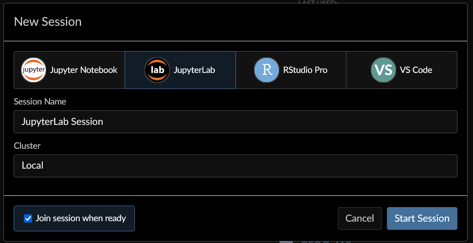
Once you are logged in, press new session and start a Jupyter Lab Session
JupyterLab
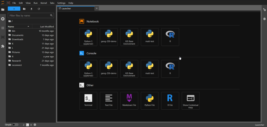
Inside of Jupyter Lab there are two main panes, the file explorer, and the Editor Pane that starts on the launcher. When creating files they will be created wherever you currently are in the file browser, this would also allow you to upload and download files if needed (Though we will talk about a better way given our unique system).
The launcher side allows us to create notebooks as well as some other options. Under Notebooks you will have a couple of options to start with, each of the icons represents an environment available to you. Additionally for this course we will be using the terminal as well. The editor pane is tabbed much like a web-browser and allows you to open different types of files at the same time in different tabs. Pressing the + will open a new launcher.
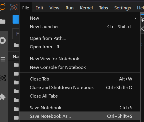
Whenever you create a new file it will be Called Untitled, as such you should make it a habit to rename files as soon as you create them, using File > Save Notebook As
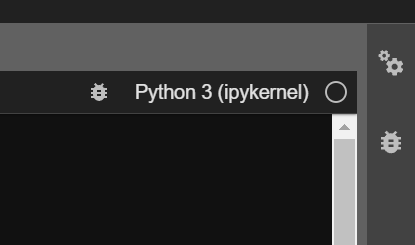
When you re-open a file it will likely not open into the environment you want, in Jupyter this is known as the Kernel, you can check your current environment by viewing the upper right corner of the editor
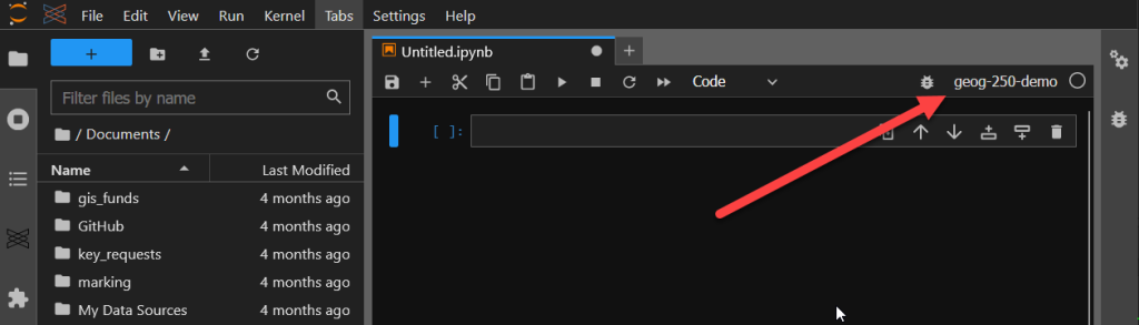
If it is not the expected kernel simply click the name, and choose the correct environment from the list provided.
Open a new tab and open a terminal
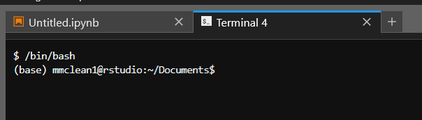
This will create a new Linux terminal, one step you will need to do after opening the terminal is to type the command “/bin/bash” and press enter, this will activate bash (Bourne Again Shell) and allow you to use tab to complete in the terminal as well as activating Anaconda our package manager. By default we are always in the base environment. The terminal will always show the following information in braces the current python environment, then your username, the server you are on, finally the file path of the current directory (note that ~ is shorthand for /home/<username> and may be used interchangeably).
GIS File System
It is important you use caution when saving files in the GIS Lab as only your K drive is backed up. Your K drive is also accessible from every GIS Computer for easy access. On windows you can find this by going to This PC and the K drive; as well as noting that the Documents, Pictures, and Downloads folders in quick access maps to K:\Documents etc.
On Linux your K drive is available at /home/<user>/K as well as the Documents, Pictures, and Download folders. In jupyter lab your default working directory is home/<user> this is not a safe place to save files so care must be used to change directory into either K or Documents.
Additionally it should be noted that we are working on a Linux server and the slashes are the opposite direction compared to windows.
Python Environments
When programming we often wish to use code written by other people that prevents the need for us to write everything on our own. We do this by importing libraries that others have published. When we download libraries they are placed into an environment. An environment is at its simplest a directory where these libraries are stored on our computer. In larger software projects it is typical for each project to have its own environment; to prevent issues with incompatible libraries (multiple definitions of the same function) or differing version requirements. Additionally it provides a simple way to share your environment with others working with you as the environment can also be defined as a text files as a list of packages and versions. This list of packages can then be reliably shared and reproduced on other computers, and in many cases even where the operating system is different.
Lets start by making an environment you will use for this course, in Jupyter Lab open a terminal, and run the command “/bin/bash” to get the full shell.
Create an environment with the name geog250-<username> for example mine will be geog250-mmclean1. We will do this with the command
conda create --name geog250-mmclean1
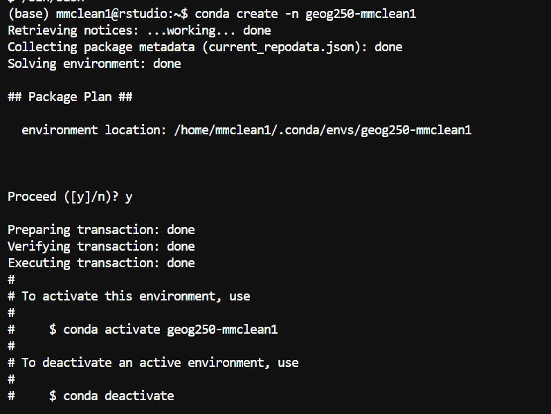
Notice that this location is not in our K drive or an otherwise redirected folder, that is OK, as none of our work goes into the environment and our code will run faster not being transferred over the network. Additionally it also gives us the code to activate the environment, you can go ahead and do this now. Making sure your console changes the start from (base) to (your new env).
Now we will install some libraries into the new environment, this is done with ‘conda install’ the first package we will install is mamba (https://mamba.readthedocs.io/en/latest/) mamba is a re-implementation of conda in c++ code instead of python, and has much faster performance in ‘solving the environment’ geospatial libraries tend to be large and have a lot of dependency issues making installing packages a time consuming process.
conda install mamba
When you run this command you will see that mamba is not found, in the current repositories. By default every anaconda environment gets the default conda repository, however some of our libraries used in this course are only available from conda-forge which is the community sponsored repositories. Additionally after we add conda-forge we will set the channel priority to strict meaning it will always take the version out of the most recently added repository if available, even if it is an older version of a package, this will help to reduce conflicts.
conda config --add channels conda-forge
conda config --set channel_priority strict
conda install mamba
Finally lets use mamba to add several other packages we will be using in the course
mamba install contextily rasterio cartopy pandas rasterstats xarray shapely pyproj gdal netcdf4 jupyter
Adding an environment to Jupyter
Before you can use your new environment inside of Jupyter you need to install the Iron Python Kernel
python -m ipykernel install --user --name=geog250-mmclean1
Once complete refresh the page, open a new launcher tab an your new environment should be an option in the Notebooks Section.
Git
When writing code we often have a desire to work in teams, and share code. This presents an interesting problem in how can many people work on the same files at the same time. This is where distributed version control systems come in. These are systems for storing in a central repository, while still having copies distributed to various users for independent modification. These systems then provide ways for compiling changes and keeping track of who changed what. Git is one such of these systems, with the most popular repository being git hub. We also maintain a repository on campus using gitlab deployed at https://git.gis.unbc.ca. Start by going to this website and logging in with your UNBC credentials.
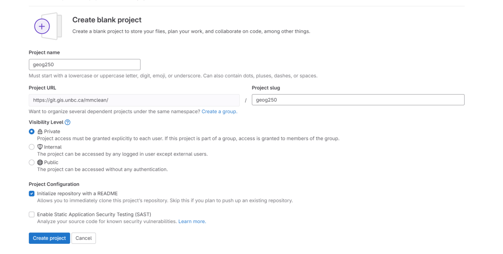
Once logged in create a project, then create a blank project.
Name your project geog250 and leave visibility to private.
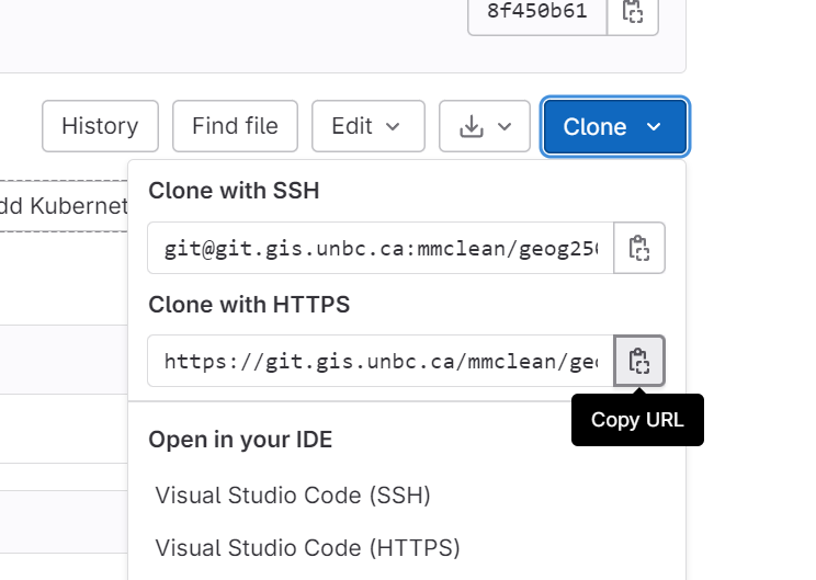
When the page loads copy the clone URL
Now in the terminal us the cd command to get into K\Documents
cd ~\K\Documents
Then clone your new repository, by using the command git clone. Note that you can paste the copied URL by pressing [Shift]+[Insert].
git clone https://git.gis.unbc.ca/mmclean/geog250.git
If you run the ls command you should see your new geog250 folder, cd into it. Then use git status
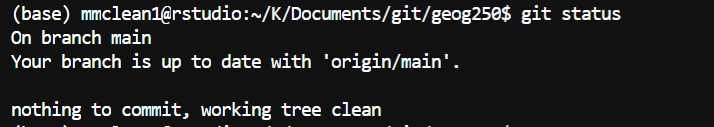
Git status, shows you what files have changed. The main git commands you will want to know are
add – a file name or -A for all files to be watched.
commit – Think of a commit as a snapshot in time that the code can be rolled back to, every commit has a message attached to it that is an opportunity to say what changed.
pull – downloads the most recent commit from the repository to your computer.
push – uploads your commits to the repository.
merge – used to combine conflicting commits, needed if two people have changed the same file.
branch – Beyond the scope of this course, but I would highly encourage further research into git.
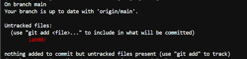
To see how this works we will create a new directory for lab00, create an empty text file inside called helloworld.txt, then check git status.
mkdir lab00
touch lab00/helloworld.txt
git status
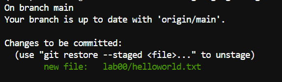
git add -A
git status
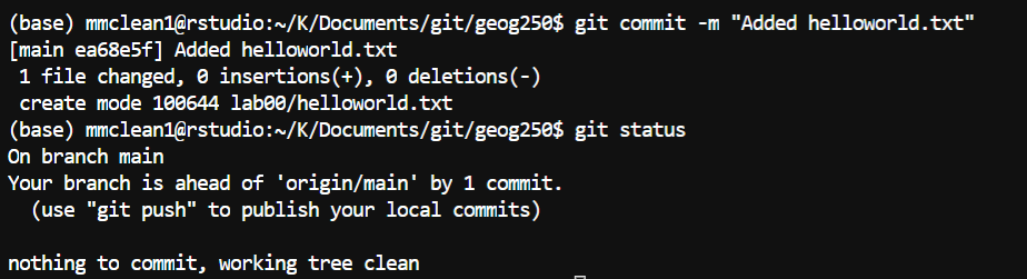
git commit -m “Added helloworld.txt”
git status
Finally use git push to upload your changes.
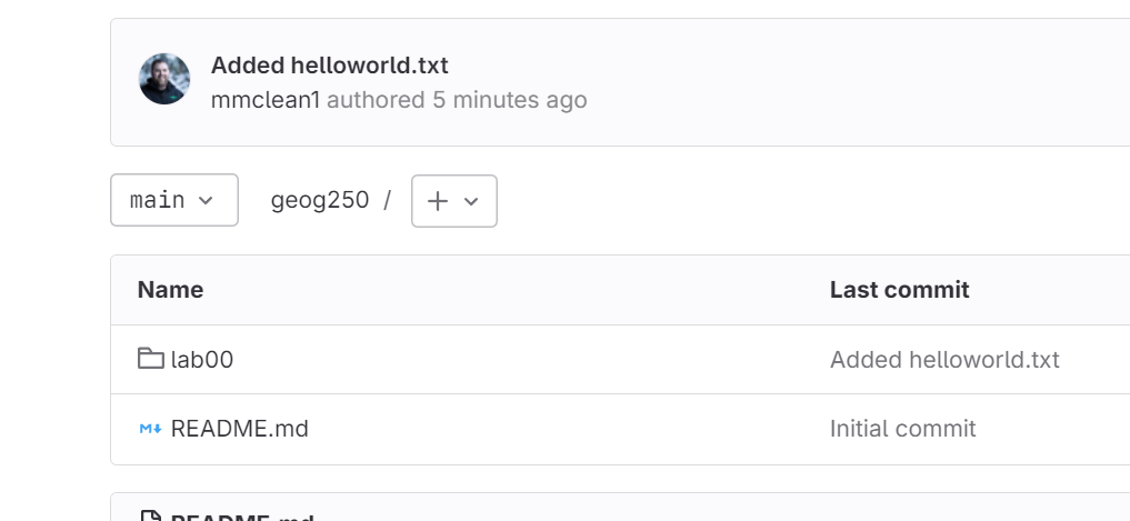
Finally go back to the gitlab website refresh, and notice the new folder is present in the code.
If you were to work on a different computer you would first ‘git pull’ to get the most recent version, do your work then commit, and push when finished.
You do not need to use for the labs however it is recommended to get practice as we will be using git in the final projects for collaboration.
At a minimum I would recommend you do all your labs in this folder and push regularly to maintain a backup.
On final order of business is to make sure we are not uploading imagery into git. In the root of the git folder you just cloned run
nano .ignore
And past the following contents, this will cause git to ignore the following file extensions.
#JupyterCheckpoints
*.ipynb_checkpoints*

#Image Files
*.TIF
*.tif
*.TIFF
*.tiff
*.ovr
*.OVR
*.aux.xml
*.jpg
*.JPG
*.JPEG
*.jpg
*.jpeg
*.PNG
*.png
*.gif
*.GIF

#ShapeFiles
*.shp
*.shx
*.dbf
*.prj
*.sbn
*.fbn
*.ixs
*.mxs
*.atx
*.shp.xml
*.cpg
*.qix
First Python Program
The first notebook you will be using is in the GEOG250 demos, you can clone this repository by cd to Documents (out of your git repository) and cloning the demos repository, new demos can be received by running git pull in the demo directory at the start of each lab.
git clone https://git.gis.unbc.ca/classes/geog-250-demos.git
Once cloned use Jupyterlab’s file browser to find and open the file 0_PythonBasics.ipynb. Once open change the kernel to the environment you just created by clicking on the upper right corner.
We will now work through the Notebook.
It is recommended you complete the Exercise notebooks as the material will be covered in Quiz 1, however no assignment is due this week.